neuPrint GUI Guide: Exploring Connectivity via the Web Browser
Exploring Neural Connectivity with neuPrint
In the previous guide, you learned how to use the Male CNS Cell Type Explorer to investigate cell types, visualize their neurons, and explore their upstream and downstream connectivity.
In fact, you have already been working with connectivity information from neuPrint! The Cell Type Explorer provides a convenient interface for exploring information derived from the male-cns:v1.0 neuPrint dataset.
Now, we are going to go directly to neuPrint itself.
This gives us access to more ways of searching for neurons, examining their connections, visualizing their anatomy, and exploring the organization of neural circuits.
1. What is neuPrint?
neuPrint is an online tool that helps scientists explore and store connectomic data. neuPrint makes it easy for anyone, from experts to students, to look at this data using a web browser. It also has tools for programmers who want to ask more complex questions. By sharing data openly, neuPrint helps speed up brain research and lets more people around the world explore how the brain is wired. This tutorial will focus on using neuPrint Explorer (the web interface) to analyze our optic lobe data
Let’s begin, click this link to the neuPrint male CNS connectome:
Open the Male CNS Connectome in neuPrint
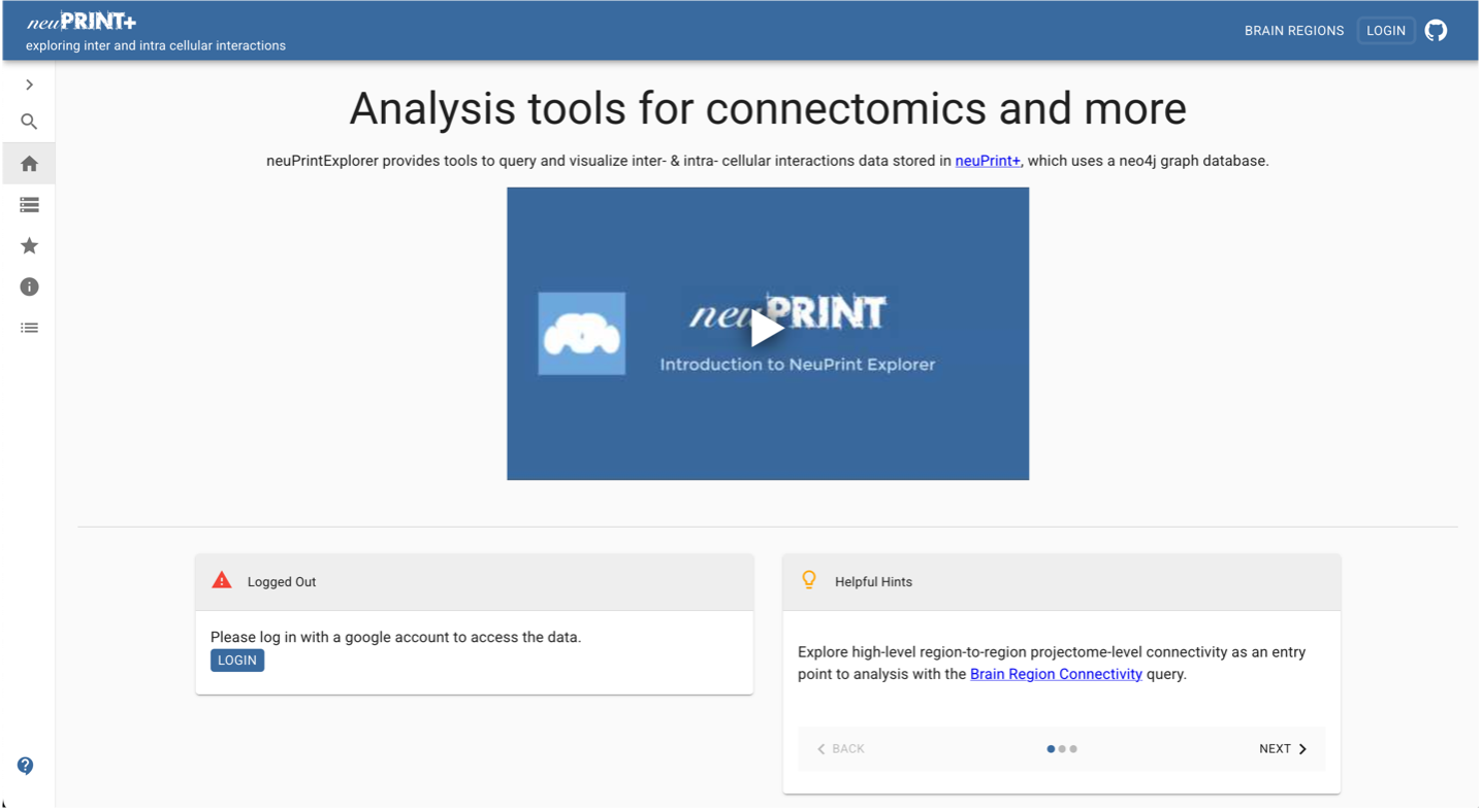
Figure 1: neuPrint Explorer. The neuPrint web interface provides tools for searching neurons, exploring their connectivity, and visualizing their anatomy within a connectome dataset.
You will have to make an account before accessing the connectome data (it’s free). Click on the LOGIN button in blue to make an account using your email (Google Account).
Once you logged in, you should reach a page that looks like the one below.

Figure 2: neuPrint Explorer after logging in.
Before searching for anything, look at the red triangle in Figure 2. This points to the dataset selector.
neuPrint contains multiple connectome datasets, so it is important to make sure you are using the correct one.
For this competition, select:
male-cns:v1.0
This is the same Male CNS dataset that you explored using the Cell Type Explorer.
Then click the “search icon” on the left hand side (see red circle, Figure 2 above) to search a neuron of your liking.
2. Finding a Neuron
Where it says “Neuron Instance, Type or BodyId (optional)” (see red rectangle, Figure 3 below), type in your neuron name (e.g., AL-MBDL1). Click SUBMIT once selected.
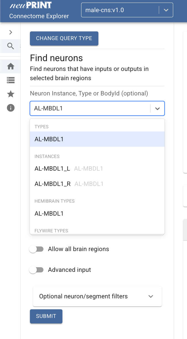
Figure 3: Searching for AL-MBDL1 in neuPrint. The Find Neurons interface allows you to search using a neuron instance, cell type, or unique Body ID.
Notice that we searched for a cell type, AL-MBDL1.
Remember from the previous guide that a cell type can contain multiple individual neurons. In this case, AL-MBDL1 contains two neurons, one associated with each side of the brain.
Click SUBMIT.
3. Understanding the Neuron Panel
Once you click submit, you should see something like this:

Figure 4: Neuron information in neuPrint. Searching for a cell type returns information about the individual neurons belonging to that type.
You’ll see a panel with information about the neuron (see below).
ID is the unique number used to identify that specific neuron.
Type is the more familiar name for the neuron (like “AL-MBDL1”).
Inputs (#post) show how many connections this neuron receives from its upstream partners.
Outputs (#pre) show how many connections this neuron sends to its downstream partners.
Brain Region Breakdown shows where in the fly brain these connections are happening, as a percentage.
Consensus NT tells us the predicted neurotransmitter the neuron likely uses to send signals.
There is an important distinction here.
AL-MBDL1 is the cell type, whereas each row represents an individual neuron with its own unique ID. This is the same distinction between cell type and individual neuron that we introduced earlier.
4. Exploring Synaptic Connectivity
Now let’s ask one of the most important questions in connectomics:
Who does this neuron connect to?
Click on the “C” icon (if you hover over it, it says Synapse Connectivity). We have pointed it out with the red arrow.

Figure 5: Opening Synapse Connectivity.
When you click it, neuPrint will show the top connections to and from your neuron of interest—AL-MBDL1 in this example—in a circular diagram:
Upstream neurons send signals to AL-MBDL1.
Downstream neurons receive signals from AL-MBDL1.
You’ll also see the identities of these connected neurons, giving you a sense of AL-MBDL1’s place in the circuit!
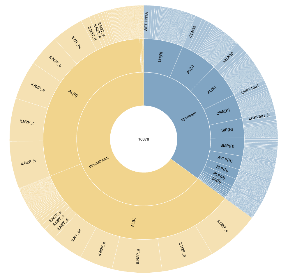
Figure 6: Synaptic Connectivity of AL-MBDL1 (ID 10378).
The neuron 10378 you selected appears at the center of the diagram.
The surrounding neurons are its synaptic partners. One side represents neurons providing input to your neuron (i.e., upstream partners), while the other represents neurons receiving its output (i.e., downstream partners).
So you can think of the diagram as:
Upstream neurons → AL-MBDL1 → Downstream neurons
The sizes of the sections help you see which partners contribute more strongly to the neuron’s connectivity. Instead of looking through a long table of connections, you can quickly identify some of its major partners.
Try clicking one of the blue sections representing the upstream side. neuPrint can then focus the visualization on the upstream partners. You can similarly explore the downstream side.
This is essentially the same concept you encountered in the Cell Type Explorer’s Connectivity tables—but now you are exploring it directly in neuPrint.
5. Visualizing the Neuron Again
Return back to the same page before you clicked the C button.
Next to the C button, you will also see an eye icon.
Click it.
A familiar interface should appear on the side:
Neuroglancer!
You have already learned how to use Neuroglancer in the Cell Type Explorer. Here, neuPrint can send the neuron you are investigating directly into Neuroglancer so that you can examine its 3D morphology.
This illustrates an important relationship between the tools:
neuPrint helps us investigate connectivity, while Neuroglancer helps us visualize the morphology.
And the two can work together.
6. Viewing a Neuron as a Skeleton
Look toward the top of neuPrint (after you clicked the eye icon to open Neuroglancer)
You should currently see a tab called:
0 - FIND NEURONS
But notice that there are also additional tabs:
1 - NEUROGLANCER
and
2 - SKELETON
Click SKELETON.
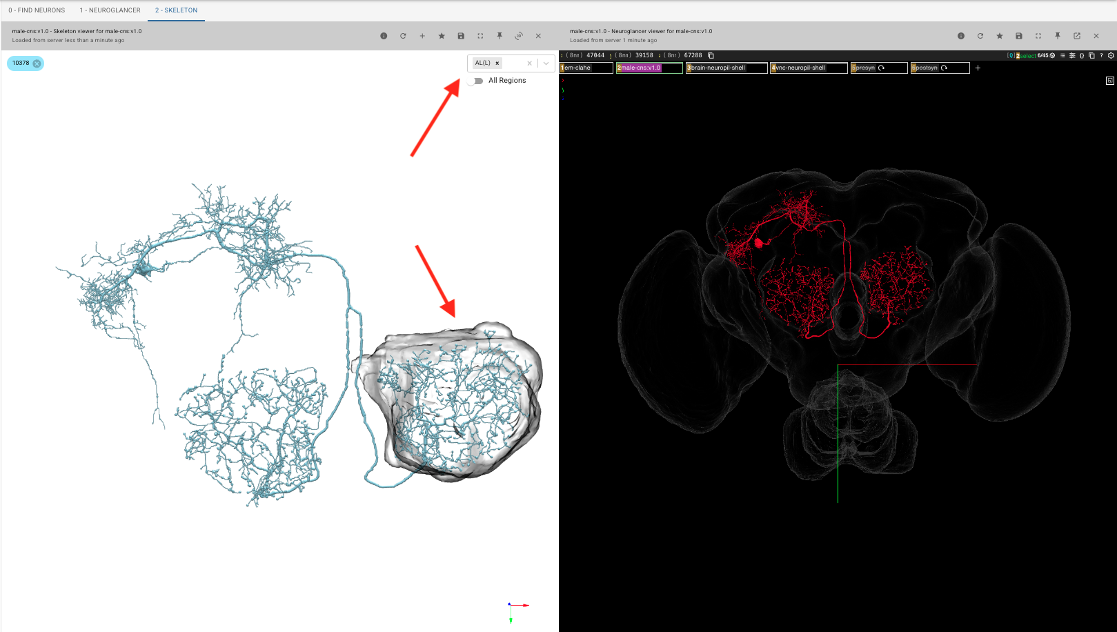
Figure 7: Skeleton visualization of AL-MBDL1.
A neuron skeleton is a simplified representation of a neuron’s shape.
Instead of displaying the full reconstructed volume of the neuron, the skeleton represents its branches as a network of lines. This makes it easier to see the neuron’s overall branching structure and trace how different parts of the neuron travel through the brain.
Pretty cool, eh?
7. Adding Neuropil Meshes
A neuron by itself can be difficult to interpret anatomically.
We might be able to see its branches—but where in the brain are those branches actually located?
To answer this, we can add a neuropil mesh.
A mesh is a 3D surface representing the approximate boundary of an anatomical structure. You have actually seen these before: the brain and neuropil surfaces displayed in Neuroglancer are examples of meshes.
Remember what we learned about AL-MBDL1 earlier. From its connectivity and brain-region information, much of its input and output is associated with the antennal lobes.
Let’s see where one of those structures is.
At the top of the Skeleton viewer, use the option for adding a neuropil mesh and select:
AL(L)
AL stands for Antennal Lobe, and (L) indicates the left side.
A gray structure should now appear around part of the neuron. This is the mesh representing the left antennal lobe.
Now the neuron’s anatomy has some context: instead of simply seeing branches floating in space, you can see how those branches relate to a particular neuropil.
Try adding another neuropil mesh.
For example, let’s investigate SIP(R) (right Superior Intermediate Protocerebrum).
From the Brain Region Breakdown in neuPrint, we can already spot something interesting:
AL-MBDL1 receives 488 input connections in
SIP(R).In contrast, it makes only 29 output connections there—even though
SIP(R)is its third-largest output region afterAL(R)andAL(L).
That is quite a striking difference: 488 inputs versus only 29 outputs.
Can we see evidence of this difference in the neuron’s anatomy?
Add the SIP(R) neuropil mesh. Then, one at a time, display:
presyn— AL-MBDL1’s presynaptic sites, where it sends outputs to downstream neurons.postsyn— AL-MBDL1’s postsynaptic sites, where it receives inputs from upstream neurons.
Before reading further, make a prediction:
Around
SIP(R), would you expect to see more presynaptic sites or postsynaptic sites?
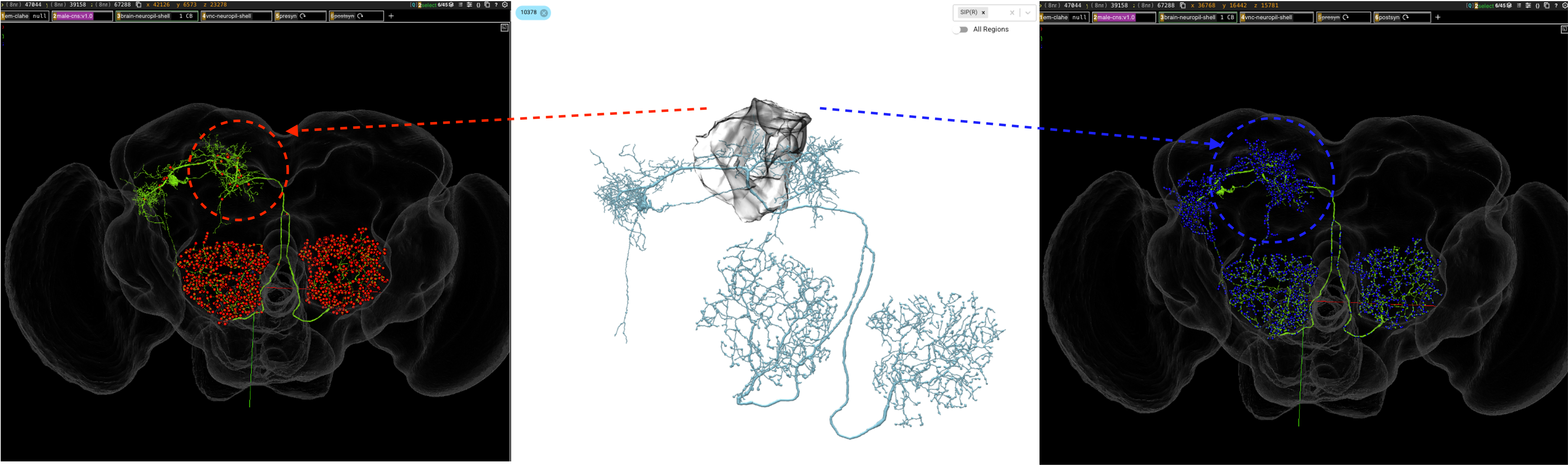
Figure 8: Comparing AL-MBDL1 inputs and outputs around SIP(R). The center panel shows the AL-MBDL1 skeleton together with the gray SIP(R) neuropil mesh. The dashed arrows indicate the corresponding SIP(R) region in the Neuroglancer views. In the left panel, the red dots show AL-MBDL1’s presynaptic sites (outputs); in the right panel, the blue dots show its postsynaptic sites (inputs). The dashed circles highlight the branches around SIP(R).
Did you notice anything?
Let’s compare the regions highlighted by the dashed circles, which is approximately where the SIP(R) is.
Around SIP(R), there are visually far more blue postsynaptic sites than red presynaptic sites. Remember:
Red presynaptic sites → where AL-MBDL1 sends information to downstream partners
Blue postsynaptic sites → where AL-MBDL1 receives information from upstream partners
This visual pattern agrees with the quantitative data from neuPrint: AL-MBDL1 has 488 input connections but only 29 output connections in SIP(R).
So two different ways of exploring the connectome are telling us the same story:
Connectivity data → many more inputs than outputs in SIP(R)
Visualization → many more postsynaptic than presynaptic sites around SIP(R)
This is a useful approach when exploring a connectome: spot an interesting pattern in the numbers, make a prediction about what you might see anatomically, and then use visualization to investigate it.
8. Putting the Tools Together
You have now investigated the same neuron in several different ways.
You used Find Neurons to identify it.
You examined its inputs and outputs.
You used Synapse Connectivity to identify its upstream and downstream partners.
You opened it in Neuroglancer to examine its 3D anatomy.
And you used the Skeleton viewer and neuropil meshes to see how its branches relate to particular brain regions.
Together, these can be combined to start asking insightful biological questions:
Where does this neuron receive information?
Where does it send information?
Which neurons provide those inputs?
Which neurons receive its outputs?
How does its anatomy allow it to connect those parts of the brain?
That is the power of connectomics: we can move from looking at a single neuron to asking how that neuron fits into a much larger neural circuit.