Male CNS Cell Type Explorer
Exploring Cell Types with the Male CNS Cell Type Explorer
In the previous guides, you learned that the male Drosophila CNS connectome contains more than 160,000 individual neurons. You also learned that neurons with similar anatomical and connectivity characteristics can be grouped into cell types.
But with thousands of cell types in the connectome, how do we actually find and explore them?
One useful starting point is the Male CNS Cell Type Explorer.
The Cell Type Explorer provides a searchable catalog of cell types in the male-cns:v1.0 dataset. It brings together information about their anatomy, neurotransmitters, brain regions, synapses, and connectivity in one interface.
Let’s explore it!
1. Open the Cell Type Explorer
Go to:
You should arrive at a page like this:
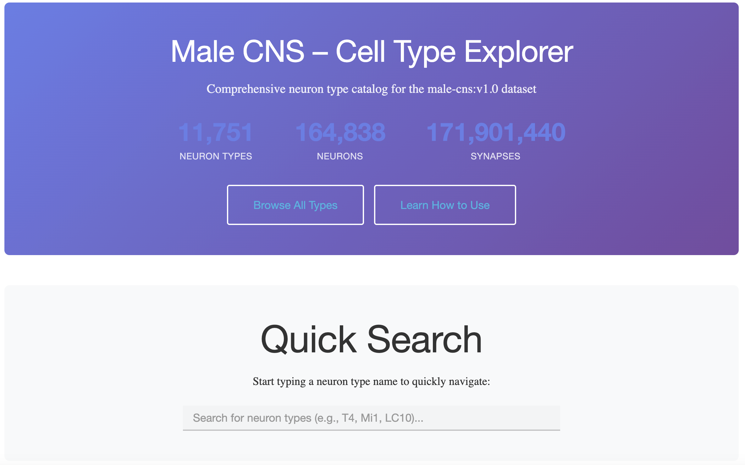
Figure 1: Male CNS Cell Type Explorer home page. The explorer provides a searchable catalog of cell types from the male-cns:v1.0 connectome dataset.
At the time this guide was prepared, and as you can see from the image above, the Cell Type Explorer contained:
164,838 neurons
11,751 neuron types
more than 171 million synapses
Because a neuron is a type of cell, in this guide the terms cell type and neuron type refer to the same concept and can be used interchangeably.
Remember the distinction from the previous guide:
One cell type ≠ one neuron.
A cell type can contain many individual neurons. For example, hundreds of individual neurons can all belong to the same visual cell type because they share characteristic anatomical and connectivity properties.
The Cell Type Explorer helps us move between these two levels: we can search for a cell type, and then investigate the individual neurons belonging to it.
2. If You Already Know a Cell Type
Sometimes you may already know what you want to investigate.
Perhaps you encountered a neuron type such as LC10a or T4 while reading a research paper. In that case, the easiest option is the Quick Search box on the home page.
For example, you have already encountered Mushroom Body Output Neurons (MBONs) in our introduction to fly neuroanatomy.
Try typing:
MBON
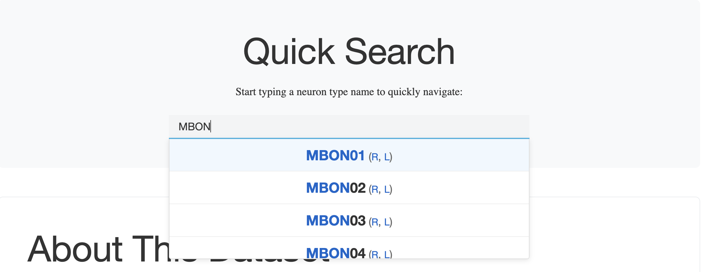
Figure 2: Searching for a known cell type. Typing MBON into Quick Search returns matching mushroom body output neuron types, such as MBON01, MBON02, and MBON03.
You can then select one of the suggested cell types to open its page.
3. What If You Don’t Know What to Search For?
You do not need to begin with a particular neuron in mind.
Sometimes the best way to start is simply to browse the connectome and see what you find.
Return to the home page and click Browse All Types.
You should see the complete Neuron Type Index:
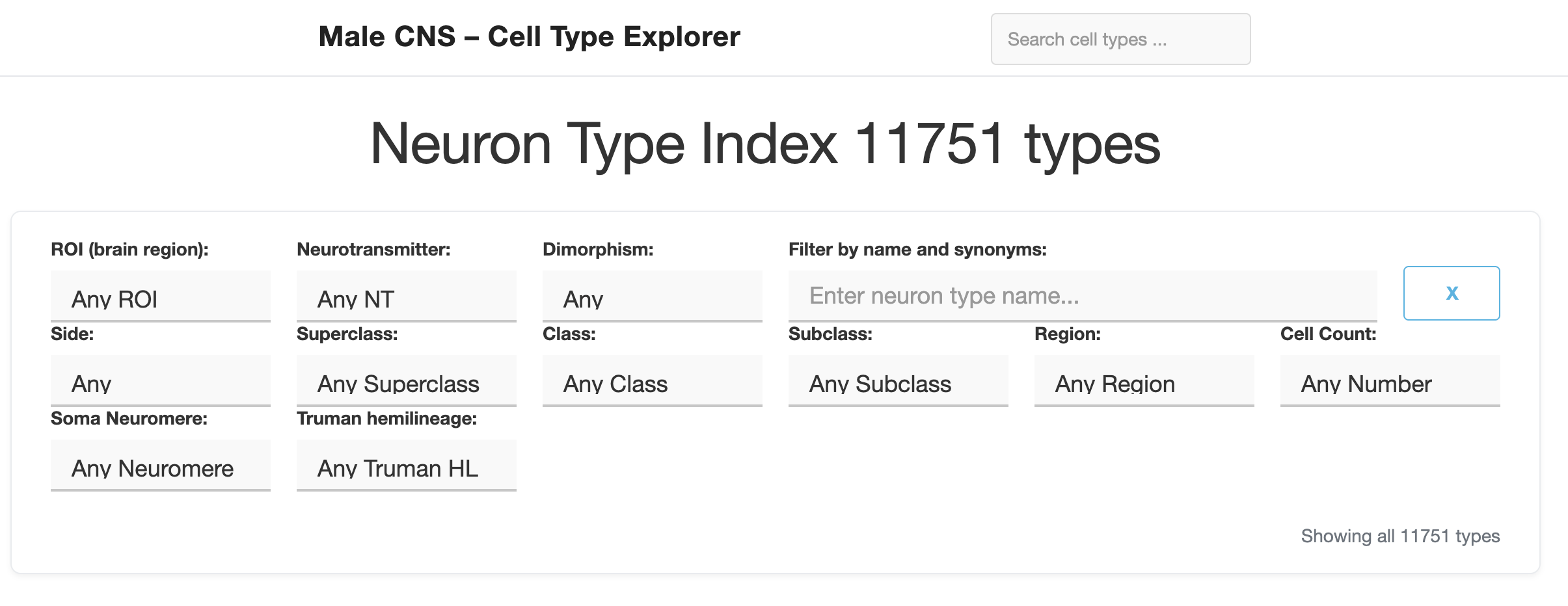
Figure 3: Neuron Type Index. The Cell Type Explorer allows you to browse thousands of neuron types and narrow them using properties such as brain region (ROI), neurotransmitter, superclass, class, subclass, and cell count.
There are lots of filters here. Don’t worry about understanding all of them yet.
A particularly intuitive place to start is with something you already know: brain anatomy.
Filtering by Brain Region (ROI)
Look at the first filter in the upper-left corner:
ROI (brain region)
ROI stands for Region of Interest. In this dataset, ROIs are anatomically defined regions of the nervous system, such as the medulla (ME), mushroom body (MB), or antennal lobe (AL).
For the Cell Type Explorer, a neuron is considered to innervate an ROI if it has synapses within that region.
For example, suppose you are interested in the mushroom body, which you learned about in the previous guide.
Click:
ROI (brain region) → MB
The explorer will now show cell types with synapses in the mushroom body.
You can combine filters later—for example, you might ask for neurons that have synapses in a particular ROI and use a particular neurotransmitter. For now, let’s just experiment with one filter.
4. Exploring a Cell Type: AL-MBDL1
Once you click choose “MB” as the ROI, you can see that there are “581 of 11751 types shown.” The first one is the AL-MBDL1 cell type.
Let’s use this particular cell type as an example throughout the rest of this tutorial:
When you open a cell-type page, the first section gives you a quantitative summary of that type.
For AL-MBDL1, you will see:
| Measure | Value | What does it tell us? |
|---|---|---|
| Neurons | 2 | There are two individual AL-MBDL1 neurons: one assigned to the right and one to the left. |
| Synapses | 18,622 | Total number of presynaptic and postsynaptic sites across the two neurons. |
| Connections | 30,127 | Total anatomical synaptic connections made with other neurons. |
| Neurotransmitter | ACh (79.4% CL) | Acetylcholine is the predicted neurotransmitter, with a reported confidence level of 79.4%. |
| Synapses per Neuron | 9,311 | Average number of synaptic sites per AL-MBDL1 neuron. |
| Connections per Neuron | 15,063.5 | Average number of anatomical connections per AL-MBDL1 neuron. |
Notice that synapses and connections are not quite the same thing.
A presynaptic release site can contact multiple postsynaptic partners. Because of this, the number of anatomical connections does not have to equal the number of presynaptic and postsynaptic sites.
From the table above the image, you will also see values for the right and left neurons and a log ratio describing how balanced the values are between the two sides. For this introductory tutorial, you do not need to calculate or interpret the log ratio in detail. Values near zero generally indicate that the two sides are relatively balanced.
Part I: Seeing the Neurons
5. Neuron Visualization with Neuroglancer
Scroll down until you reach Neuron Visualization.
This is not simply a static image. The Cell Type Explorer has embedded another tool inside the page:
Neuroglancer.
Neuroglancer allows us to interact with the reconstructed neurons in 3D.
For AL-MBDL1, the viewer initially shows the two individual neurons belonging to the cell type—one on each side of the brain.
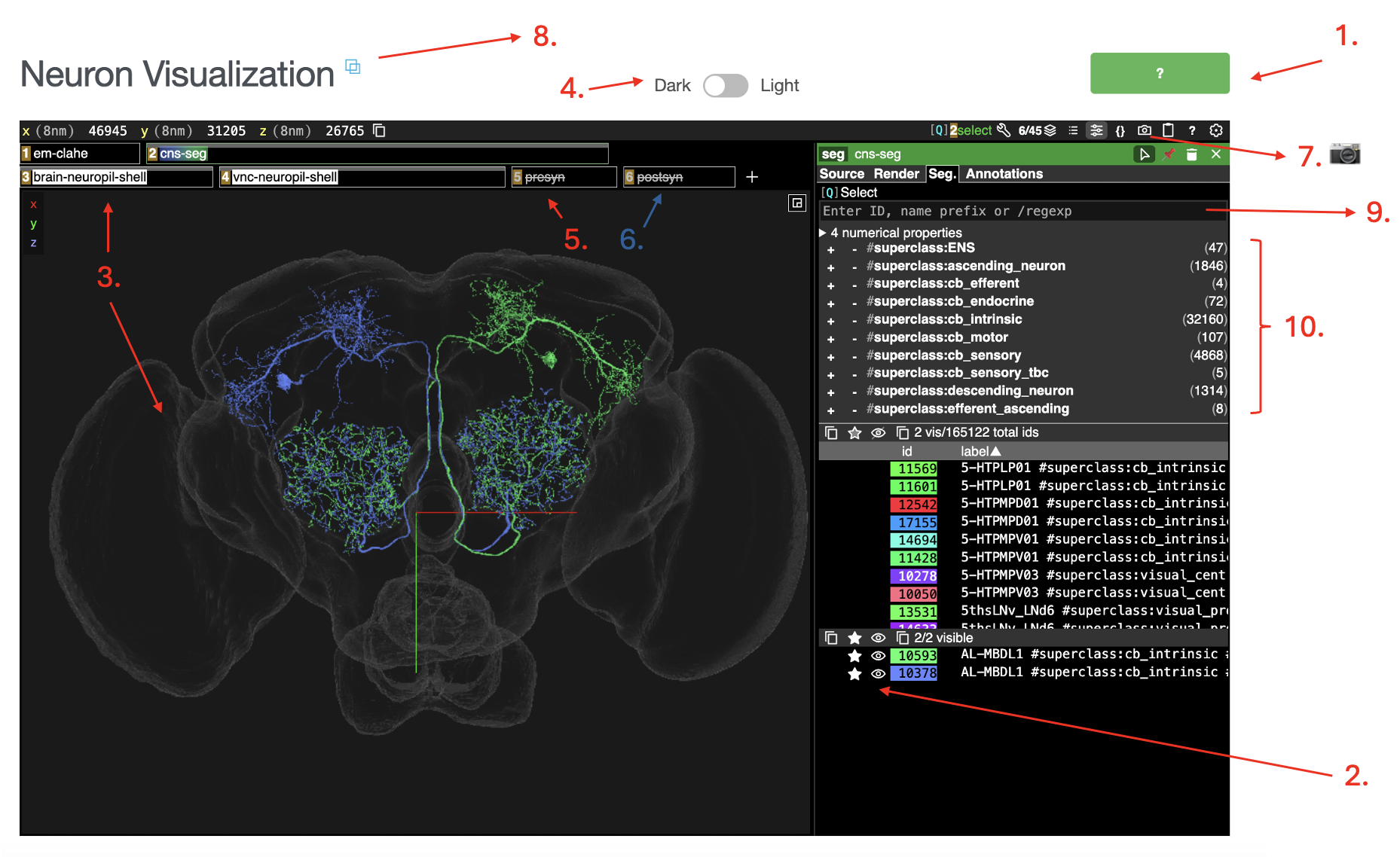
Figure 4: Exploring AL-MBDL1 with Neuroglancer. The Cell Type Explorer includes an embedded Neuroglancer viewer for interactively examining the 3D anatomy of neurons. Numbered arrows indicate several useful controls described below.
Let’s experiment with it.
1. Learn the Navigation Controls
Hover over the green ? button.
This displays instructions for navigating the 3D viewer.
Try:
clicking and dragging to rotate the brain;
holding Shift while dragging to move the view;
zooming in and out;
pressing
zto reset to the closest viewing axis;pressing
oto switch between orthographic and perspective views; andpressing
lto assign new random colors to the neurons and ROI meshes.
The goal is simply to become comfortable moving around a reconstructed brain.
2. Show and Hide Individual Neurons
Look at the list of AL-MBDL1 neurons on the right.
The eye icon controls whether each neuron is visible.
Try hiding one AL-MBDL1 neuron and leaving the other visible.
Remember: these are two individual neurons belonging to the same AL-MBDL1 cell type.
3. Remove the Brain Neuropil Shell
At the top-left, find:
brain-neuropil-shell
Turn this layer off.
Notice what changes.
The gray brain outline provides anatomical context, but hiding it can make the morphology of individual neurons easier to inspect.
4. Change the Theme
Try switching between Dark and Light mode.
This does not change the data. It only changes how the viewer is displayed.
5. View Presynaptic Sites
Turn on:
presyn
Small markers (as red dots) will appear at the neuron’s presynaptic sites.
Recall from the anatomy guide: these are locations where the neuron provides output to postsynaptic partners.
6. View Postsynaptic Sites
Now turn on:
postsyn
These markers (as dark blue dots) indicate postsynaptic sites, where the neuron receives inputs from other neurons.
Try comparing where the presynaptic and postsynaptic sites occur along the neuron’s branches.
7. Take a Screenshot
Click the camera icon.
You can use the default settings and select Take screenshot to capture the current Neuroglancer view.
This can be useful when documenting interesting neurons or preparing figures for your project.
8. Open the Full Neuroglancer Viewer
Next to Neuron Visualization, click the double-square icon.
This opens the visualization in a full Neuroglancer window.
You may then realize that Neuroglancer is its own visualization tool.
The Cell Type Explorer has simply made it convenient by embedding a Neuroglancer view for the cell type you are currently investigating.
9. Search for Other Neurons
In the full viewer, you can search for neurons using identifiers or names in the search field.
For now, it is often easier to begin with the Cell Type Explorer and let it open the relevant neurons for you.
10. Filter Neurons
You may also notice filters such as:
#superclass:...
These allow you to search broader groups of neurons—for example, using the superclasses introduced in the previous guide.
Again, don’t worry about mastering these filters yet.
6. Why Visualize a Neuron?
At this point, you might reasonably ask:
Why do we need to look at the neuron’s shape at all?
A neuron’s morphology can provide important clues about what it might be doing.
Ask yourself:
Which neuropils does the neuron enter?
Where does it branch most extensively?
Does it remain on one side of the brain or cross the midline?
Where are most of its postsynaptic input sites?
Where are most of its presynaptic output sites?
Does it appear to carry information from one brain region to another?
For example, if a neuron receives many inputs in one neuropil but provides many outputs in another, that might suggest that it helps transfer or transform information between those regions.
Part II: Where Does the Cell Type Connect?
7. ROI Innervation
Immediately below the visualization, you will find the ROI Innervation table.
Remember that an ROI is a Region of Interest—an anatomically defined part of the nervous system.
For AL-MBDL1, the page reports synapses across 22 ROIs.
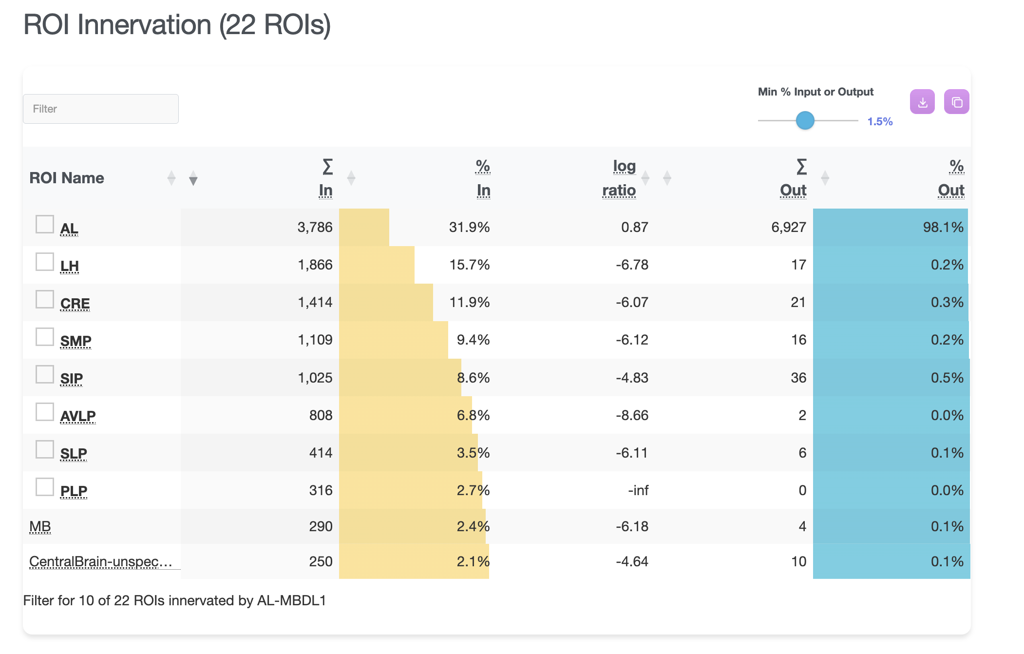
Figure 5: ROI Innervation for AL-MBDL1. The table summarizes how the input and output synapses of AL-MBDL1 are distributed across different anatomical regions of the nervous system.
What Does “22 ROIs” Mean?
It means that AL-MBDL1 has synapses within 22 anatomically defined regions represented in the dataset.
However, Figure 5 only displays 10 of them.
Why?
Look at the slider labeled:
Min % Input or Output
It is currently set to 1.5%.
This means the table only shows ROIs that contain at least 1.5% of the cell type’s total inputs or at least 1.5% of its total outputs. For example, if an ROI contains only 1% of AL-MBDL1’s total inputs and 0.9% of its total outputs, it will not appear at this threshold.
Understanding the Columns
Let’s use the first row, AL, as an example.
AL stands for Antennal Lobe.
| Column | Meaning |
|---|---|
| Σ In | Total number of input connections received by the cell type you are exploring within that ROI |
| % In | Percentage of all input connections received by the cell type you are exploring that occur within that ROI |
| log ratio | Indicates whether the cell type you are exploring has relatively more outputs or inputs within that ROI |
| Σ Out | Total number of output connections sent by the cell type you are exploring within that ROI |
| % Out | Percentage of all output connections sent by the cell type you are exploring that occur within that ROI |
For the antennal lobe (AL), Figure 5 shows:
3,786 inputs — 31.9% of AL-MBDL1’s total inputs
and
6,927 outputs — 98.1% of AL-MBDL1’s total outputs
This immediately gives us anatomical information about the cell type.
Nearly all of its output is concentrated in the antennal lobe, while its inputs are distributed much more broadly across several regions.
What Does the Log Ratio Mean?
The log ratio summarizes whether an ROI contains relatively more input or output.
Negative value → more input than output
Positive value → more output than input
Near zero → more balanced
You do not need to calculate this yourself. Think of it as a quick way of spotting whether a brain region is predominantly an input region or output region for the cell type.
This can help you start forming hypotheses about how information flows through the neuron.
Part III: Who Does the Cell Type Connect To?
8. Connectivity
Knowing where a neuron forms synapses is useful.
But connectomics lets us ask another fundamental question:
Who is on the other side of those synapses?
Scroll to the Connectivity section.
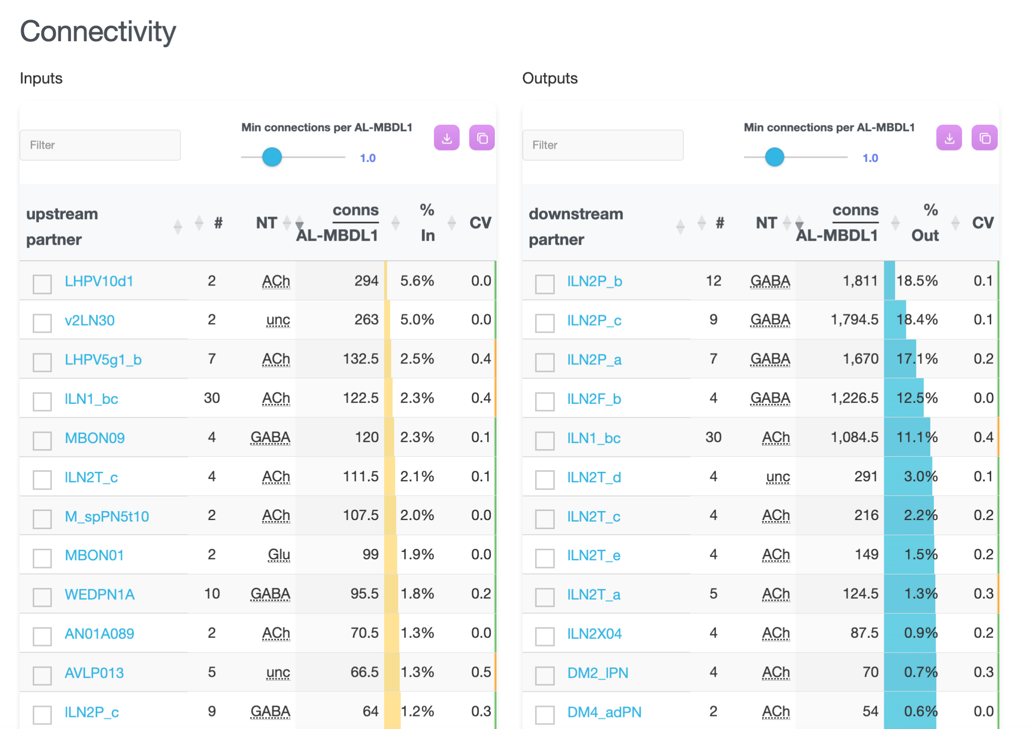
Figure 6: Connectivity of AL-MBDL1. The Inputs table shows upstream cell types that provide synaptic input to AL-MBDL1, while the Outputs table shows downstream cell types that receive synaptic output from AL-MBDL1.
The table is divided into two sides:
Inputs → Who sends information to AL-MBDL1? Neurons that SEND information TO AL-MBDL1 are called AL-MBDL1’s upstream partners.
Outputs → Who receives information from AL-MBDL1? Neurons that RECEIVE information FROM AL-MBDL1 are called AL-MBDL1’s downstream partners.
In other words, Upstream partner → AL-MBDL1 → Downstream partner
Reading the Inputs Table
Let’s look at the first upstream partner shown:
LHPV10d1
The row contains several pieces of information.
| Column | What it means |
|---|---|
| upstream partner | Cell type providing synaptic input to AL-MBDL1 |
| # | Number of individual neurons of that cell type that are upstream partners of AL-MBDL1 |
| NT | Predicted neurotransmitter used by that upstream partner cell type |
| conns AL-MBDL1 | Mean number of synaptic connections from that upstream cell type to each AL-MBDL1 neuron |
| % In | Percentage of AL-MBDL1’s total input connectivity contributed by that upstream cell type |
| CV | How variable the connection count is across the individual AL-MBDL1 neurons |
For LHPV10d1, the table shows:
# = 2NT = AChconns AL-MBDL1 = 294% In = 5.6%CV = 0.0
So LHPV10d1 is an upstream partner of AL-MBDL1. Its neurons are predicted to use acetylcholine (ACh), and connections from this cell type account for about 5.6% of the input connectivity received by AL-MBDL1.
Exploring the Data (Example)
Now let’s experiment with the connectivity table for the upstream partner of the same AL-MBDL1 cell type.
Try clicking the # column to sort it from highest to lowest. One of the cell types that stands out is ORN_DM1:
ORN_DM1: # = 37
This means that 37 individual ORN_DM1 neurons are upstream partners of AL-MBDL1.
But if you explore the ORN_DM1 cell type itself, you will find 74 ORN_DM1 neurons in total. In other words, not every ORN_DM1 neuron provides input to AL-MBDL1—only 37 of the 74 do.
Already, we have discovered something interesting!
Now try sorting by % In instead.
Although ORN_DM1 has the largest number of individual neurons providing input among these partners (37 neurons), together they account for only 0.9% of AL-MBDL1’s inputs.
Compare this with LHPV10d1:
LHPV10d1: # = 2, % In = 5.6%
There are only two LHPV10d1 neurons providing input to AL-MBDL1, yet together this cell type accounts for 5.6% of AL-MBDL1’s inputs—much more than the 37 ORN_DM1 neurons.
Why might two neurons contribute more connectivity than 37 neurons?
That’s a question worth exploring!
Reading the Outputs Table
The same logic applies on the right, except now we are looking in the opposite direction.
For example, lLN2P_b appears as a major downstream partner.
This means:
AL-MBDL1 → lLN2P_b
AL-MBDL1 provides synaptic output to neurons of this cell type.
The % Out column tells us how much of AL-MBDL1’s total output connectivity goes to that downstream cell type.
In Figure 6, the first few downstream partners each account for a substantial fraction of AL-MBDL1’s outputs. This suggests that its output connectivity is strongly concentrated onto particular cell types.
What Is CV?
CV stands for coefficient of variation.
Remember that AL-MBDL1 contains two individual neurons. Even though they belong to the same cell type, their exact connection counts do not have to be identical.
CV gives us a simple measure of how variable the connection strength is across the individual neurons of the target cell type.
As a rough intuition:
CV near 0 → relatively consistent connectivity
larger CV → more variation between individual neurons
You do not need to calculate CV yourself for this tutorial. It becomes more useful when comparing cell types that contain many individual neurons.
Adjusting the Connectivity Threshold
At the top of each table is:
Min connections per AL-MBDL1
Increasing this threshold removes weaker partners and lets you focus on stronger connections.
This can be useful because a connectome may contain many weak connections. Depending on your research question, you may want to begin by examining the cell types that contribute the largest fractions of a neuron’s inputs or outputs.
9. From Anatomy to a Circuit
We have now asked three different questions about the same cell type:
What does it look like? → Neuroglancer
Where does it form synapses? → ROI Innervation
Which cell types does it connect to? → Connectivity
These questions are much more powerful when considered together.
Suppose you discover that a neuron:
receives many inputs in one neuropil;
sends most of its outputs in another neuropil; and
receives those inputs from a particular group of upstream cell types.
You can begin developing a hypothesis about how information might flow through that neuron and what circuit it participates in.
That is one of the key ideas of synapse-level connectomics:
Anatomy + synapse location + connectivity → clues about neural circuits
But remember: the connectome tells us about anatomical connectivity. Although structural information often reveals much about its function, it does not, by itself, tell us everything about neural activity, causation, or behavior. Those questions often require computational modeling and/or additional experiments.
10. Where Does All This Data Come From?
The Cell Type Explorer makes these data much easier to browse.
Behind the scenes, the site is connected to the male-cns:v1.0 dataset in neuPrint.
neuPrint is the database and analysis platform containing the connectome data used to generate much of what you see here. This includes information about neurons, synapses, ROIs, and connectivity.
For now, the Cell Type Explorer gives us a convenient graphical way to begin exploring those data.
Later, we will go directly into neuPrint, where you will have much more control over the questions you can ask of the connectome.