1b) The Connectome Interpreter Tutorial - Linear Methods (Path-finding and Hexmaps)
Setup
Before starting this notebook, install pyvis for interactive plots:
pip install pyvisThis tutorial is adapted from the Linear Methods tutorial notebook from Connectome Interpreter. For additional information about the functions used in this tutorial, see the Connectome Interpreter documentation.
# 1. load your packages and directory paths at the top
import pandas as pd
project_dir = '/Users/aarushivardhan/Desktop/MB'
from connectome_interpreter import *

# Get cell types function list.
sheet_id = "1VHCEnurOdb4FDC_NUKZX_BpBckQ9LpKxv0CsK_ObVok"
url = f"https://docs.google.com/spreadsheets/d/{sheet_id}/export?format=csv&gid=0"
df = pd.read_csv(url)
df = df.rename(columns={'función conocida': 'known_function'}) # run this only if the column is called "función conocida", otherwise leave it out
type_to_function = dict(zip(df["cell_type"], df["known_function"])) # type_to_function contains a list of cell types and their experimentally-tested functions.


# load meta data male cns connectome
mcns_meta = pd.read_csv(
    'https://raw.githubusercontent.com/YijieYin/connectome_data_prep/refs/heads/main/data/maleCNS/mcns_all_neuron_meta.csv',
    index_col=0, low_memory=False
)
mcns_inprop = sp.sparse.load_npz(project_dir + '/mcns_inprop_all_neuron.npz') # input proportion df male cns
mcns_meta['known_function'] = mcns_meta.cell_type.map(type_to_function).fillna('') # assign known function dictionary to a column in meta df
Path Finding
Let’s say now that you have explored effective connectivity, which is essentially the influence from a source to a target neuron or cell type, your new curiosity is to explore who are those intermediate cell-types playing a role in this influence?
Path finding might be the tool you are look for as it asks: what are the paths that connect a source and target? And, which intermediate neurons carry information between a source and target?
Here, path length means the number of synaptic steps between the source and target neurons. For example, a path length of 1 means that the source connects directly to the target, while a path length of 2 means that there is one intermediate neuron between them.
This is how the paths between source and targets are computed:
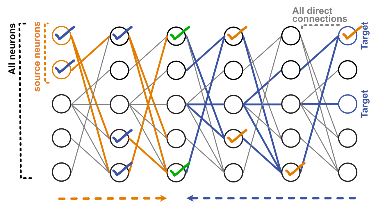
Figure 1: Finding the paths between source and target neurons. The find_paths_of_length() function looks for the intermediate neurons that connect a source neuron to a target neuron. The search starts from both ends. (1) Start from the source neurons and follow their downstream connections. These are shown in orange. (2) Start from the target neurons and work backwards through their upstream connections. These are shown in blue. (3) Where the two searches meet, you have found an intermediate neuron that can connect the source to the target. These are marked with the green ticks. (4) The function then traces these selected neurons and connections back to the original source and target, identifying the complete paths. All neurons with ticks are selected. Adapted from Yijie Yin, 2024. (You may note we have used this find_paths_of_length() in our previous tutorial for before calculating effective connectivity. Now we are diving in more detail about it works and how we can take it one step further to see the cell types that make up the path!)
Before we figure out which cell types are involved in these paths, we first need to determine the path lengths through which the source neurons influence the target neurons and look at where this influence is concentrated.
So how does one figure out the path length at which the source neuron has the greatest influence on the target neuron?
The conn_by_path_length() function calculates the connection strength across different path lengths and displays the result as an interactive line plot. The plot shows the connection strength from all of our source neurons (inidx) to the average target neuron (outidx) at each path length. This allows us to see how the connection strength is distributed across the network. For example, we might see that the connection strength is highest at path length 2, suggesting that the strongest influence in this analysis occurs through two synaptic steps. We can then use the path length with the greatest connection strength to investigate which intermediate cell types form those paths.
Let’s now pick two cell types as our source (Mi1) and target (T4a) to play with these functions!
# Let's investigate connections from Mi1 → T4a.
# Mi1: is a medulla intrinsic cell type in the visual system. It is part of the ON motion pathway.
# T4a: a motion neuron of the ON pathway responsible for detecting front-to-back motion.

# Select all Mi1 neurons whose cell bodies are on the right side.
source_idx = mcns_meta.idx[(mcns_meta.cell_type == 'Mi1') & (mcns_meta.somaSide == 'R')]

# Select all T4a neurons to use as our target population.
target_idx = mcns_meta.idx[(mcns_meta.cell_type == 'T4a') & (mcns_meta.somaSide == 'R')]

# Let's also make a dictionary that links each neuron index (idx) to its cell type and the side of the brain where its cell body is located (R/L).
mcns_idx_to_type_side = dict(zip(mcns_meta.idx, mcns_meta.cell_type + ' ' + mcns_meta.somaSide))
Right or Left or Both?
For example, we could investigate:
Right Mi1 → all T4a
All Mi1 → right T4a
Right Mi1 → right T4a
For our example, we restrict both Mi1 and T4a to the right side because it is well-known via anatomy in the literature that Mi1 and T4a are intrinsic neurons within each optic lobe and their connections are also confined to each lobe, so in this example, we are interested in the connections within the right optic lobe.
However, this is not a general rule that source and target neurons must be on the same side. Some neurons make connections across the two sides of the brain. For example, H1 neurons connect between the two optic lobes. Therefore, we should not automatically assume that a right-sided source can only connect to right-sided targets.
In the connectome-interpreter example, the authors initially use all MBON32 neurons as the source, but restrict the target to right-sided DNa03 neurons:
src_idx = fafb_meta.idx[
    fafb_meta.cell_type == 'MBON32'
]

tgt_idx = fafb_meta.idx[
    (fafb_meta.cell_type == 'DNa03') &
    (fafb_meta.side == 'right')
]
There is one MBON32 and one DNa03 neuron for the left and right side of the brain. The MBON32 right and left neurons connect to DNa03 right and left neurons, there is not separation based on hemisphere. The authors first restrict the target to right-sided DNa03 neurons because this defines the specific source-to-target connection they want to investigate.
For now let’s move on the figuring out the path length at which the source neuron has the greatest influence on the target, we will revisit this topic again shortly after fulfilling this criteria.
As a sanity check, check how many values I have in my source_idx. Since, I specficied the Mi1 neurons -> Mi1_R the cell type count should match that of cell type explorer’s value for Mi1 R. If we didn’t the value would be of the cell type population of Mi1 R and L.
len(source_idx)
# Counts how many Mi1 neurons we selected.
# This should match the Mi1 neuron count shown in the Male CNS Cell Type Explorer.887Now, let’s run conn_by_path_length which will help us figure out the path at which the source neuron exerts the greatest influence “effective connectivity” towards the target.
# Reminder: always make a habit of reading the Connectome Interpreter documentation.
# You can find a link to the documentation in the setup section of this tutorial.

# mcns_inprop: input-normalised connectivity between presynaptic and postsynaptic cell types
# source_idx: the source neurons (their row numbers in mcns_meta)
# target_idx: the target neurons (their row numbers in mcns_meta)
# n=5: we are considering connectivity across 5 synaptic hops between the source and target
# out_idx_map: groups output neurons by cell type and side. Note: you can only use either out_idx_map or in_idx_map at a time. See below for more details.

fig = conn_by_path_length(mcns_inprop, source_idx, target_idx, n=5, outidx_map=mcns_idx_to_type_side)
fig.show() #line plot version
20%|██ | 1/5 [00:01<00:06, 1.52s/it]GPU not available, using CPU instead.
40%|████ | 2/5 [00:04<00:07, 2.38s/it]GPU not available, using CPU instead.
60%|██████ | 3/5 [00:11<00:08, 4.36s/it]GPU not available, using CPU instead.
80%|████████ | 4/5 [00:30<00:10, 10.36s/it]GPU not available, using CPU instead.
100%|██████████| 5/5 [06:00<00:00, 125.59s/it]GPU not available, using CPU instead.
100%|██████████| 5/5 [06:00<00:00, 72.14s/it]
The conn_by_path_length() function’s output above shows the effective connectivity between our source and target populations at different path lengths.
Path length 1 → direct source → target
Path length 2 → source → intermediate → target
Path length 3 → source → intermediate → intermediate → target
The value at each path length represents the connectivity reaching the target through paths of that length.
This plot therefore helps us identify which path lengths contribute most to the effective connectivity between our source and target populations. Most of the connectivity seems to be concentrated at 3 hops (there is a peak there), so we will use that to see what cell types are involved in these paths.
Revisting the right and left conversation
As mentioned earlier, let’s revisit our discussion about The Connectome Interpreter’s MBON32->DNa03 example in their notebook and the use of specifying right and left. As mentioned, the authors first restrict the target to right-sided DNa03 neurons because this defines the specific source-to-target connection they want to investigate. When using conn_by_path_length(), the author separates the MBON32 source neurons according to their side.
This is because conn_by_path_length() allows you to group either the source or target neurons, but not both at the same time. By grouping MBON32 neurons by side, the authors can compare the effective connectivity from the right MBON32 and left MBON32 across different path lengths. See here.
They find that the two MBON32 neurons show the same path-length cutoff. In other words, the range of path lengths that contributes to the connectivity is consistent for both the right and left MBON32 neurons.
This observation is important for the next stage of the analysis. Since both MBON32 neurons show the same path-length pattern, and because they are connected to one another, the authors keep the same hop-cutoff for both left and right MBON32 neurons when identifying the cell types involved in the paths.
The important point is that the left/right separation here is a way of examining the results, rather than a requirement that the two hemispheres form independent pathways. Separating MBON32 by side allows the authors to check whether the two neurons behave differently. Once they find the same path-length cutoff, they retain both sides so that legitimate cross-hemispheric paths are not excluded from the downstream analysis.
Note: In the connectome-interpreter example, the authors are using FAFB, the female adult fly brain connectome aka: the FlyWire connectome.
Let’s find out who are the cell types in the intermediate?
Since for our Mi1-T4a example we have found that most connecitvity is concentrated at 3 hops, we will now use the find_paths_of_length() to get 3-hop away connections between Mi1 and T4a via the method explained in Figure 1.
# 3 hop connections from source -> target
paths = find_paths_of_length(mcns_inprop, source_idx, target_idx, target_layer_number=3)
pathsOur connections are currently organised by individual neurons. Let’s group these neurons by their cell type and soma side (right/left). As a note:
outprop=False (default) → measures input proportion: how much input the target receives from the source/path.
outprop=True → measures output proportion: how much output the source sends through the path to the target.
The combining_method parameter tells the function how to combine the values across neurons of the same cell type. We will use the default, mean, which gives us the average value across neurons in the same group.
For our Mi1 → T4a example, we use outprop=False because we are interested in how much input T4a receives from Mi1. outprop=False is the default, so we don’t have to specify it, but I did here just to illustrate this.
Remember, in your own projects, don’t blindly copy what the tutorial says. Please read the function documentation carefully and understand the parameters. For instance, if you were interested in how much output Mi1 sends to T4a, then it would be important to change the parameter to outprop=True.
paths_typed = group_paths(paths, pre_group=mcns_idx_to_type_side, post_group=mcns_idx_to_type_side, combining_method='mean', outprop=False)
paths_typedLet’s remove weak connections from our path data. I chose a weight threshold of 5%. This is arbitrary, and this threhold is used only for visualization and does not imply a biological cutoff.
# Here, weight represents the mean input proportion to a postsynaptic neuron which we did in our previous function.
# We keep only connections with a mean weight of at least 5% (0.05).
paths_filt = filter_paths(paths_typed, threshold=0.05)
paths_filtPlotting the paths
Now we can visualize the 3-hop paths between our source and target cell types.
Because our analysis is aggregated by cell type and soma side, the nodes that are in the plot will represent cell types and each edge (or line) represents a connection between two cell types along the identified paths with thickness of the edge being the input proportion strength between two cell types.
For more options for customizing the path visualization, see the plot_paths() documentation.
Adding information to the plot
If you look at the documentation above, there are all sorts of optional things you do to amp up your plot. For my case, I’m curious about the neurotrasnmitter identity (NT) of these inbetween cell types.
Using neuron_to_color, we will color each cell type according to its neurotransmitter identity. First, we create a dictionary linking each cell type and soma side to its NT as seen below:
mcns_type_side_to_nt = dict(zip(mcns_meta.cell_type + ' ' + mcns_meta.somaSide, mcns_meta.top_nt))
mcns_type_side_to_nt
# Next, we define which color should represent each neurotransmitter:
nt_to_color = {
"gaba": "blue",
"acetylcholine": "red",
"glutamate": "green",
"dopamine": "purple",
"unclear": "grey",
"octopamine": "pink",
"serotonin": "orange",
"histamine": "yellow"
}We can then use these two dictionaries to create a final dictionary required by plot_paths(). plot_paths() expects the dictionary to map each neuron identifier (cell type in our case) directly to a color, so we will convert our cell-type → NT mapping and NT → color mapping into a: cell-type → color mapping
neuron_to_color = {}
for cell_type, nt in mcns_type_side_to_nt.items():
    neuron_to_color[cell_type] = nt_to_color[nt]
neuron_to_color
{'DNp01 R': 'red',
 'OCG01d L': 'red',
 'VCH R': 'blue',
 'AOTU019 R': 'blue',
 'VS L': 'red',
 'CT1 L': 'blue',
 'DNp01 L': 'red',
 'OA-AL2i1 L': 'grey',
 'VS R': 'red',
 'MBON01 R': 'green',
 'HSN R': 'red',
 'HSE R': 'red',
 'AMMC-A1 L': 'red',
 'LAL138 L': 'blue',
 'H2 L': 'red',
 'CB2049 L': 'red',
 'HSS R': 'red',
 'H2 R': 'red',
 'DNp18 R': 'red',
 'VCH L': 'blue',
 'LoVC16 R': 'green',
 'pIP1 L': 'red',
 'AOTU041 R': 'blue',
 'GNG116 L': 'blue',
 'DNg56 R': 'blue',
 'HSE L': 'red',
 'AstA1 L': 'blue',
 'pIP1 R': 'red',
 'VL2a_adPN R': 'red',
 'Dm17 L': 'green',
 'OA-VUMa1 M': 'pink',
 'vCal2 L': 'green',
 'ER5 L': 'blue',
 'SMP108 L': 'red',
 'DNg100 L': 'red',
 'MeVC11 L': 'red',
 'MNx02 L': 'grey',
 'DNp18 L': 'red',
 'VA7m_lPN L': 'red',
 '5-HTPMPV03 R': 'orange',
 'Li39 L': 'blue',
 'LoVC14 L': 'blue',
 'DNpe013 R': 'red',
 'DNg100 R': 'red',
 'mALD1 R': 'blue',
 'DNp20 R': 'red',
 'MeVPOL1 L': 'red',
 'DCH L': 'blue',
 'DNp27 R': 'red',
 'DNb05 R': 'red',
 'LPi21 R': 'blue',
 'MeVPLp1 L': 'red',
 'DNp30 R': 'green',
 'AN07B004 R': 'red',
 'AOTU019 L': 'blue',
 'AN12B011 L': 'blue',
 'OA-AL2i1 R': 'grey',
 'PVLP010 L': 'green',
 'DA1_lPN L': 'red',
 'OCG01b R': 'red',
 'dCal1 L': 'blue',
 'MeVC1 L': 'red',
 'MBON06 R': 'green',
 'OA-VUMa3 M': 'pink',
 'OCG01b L': 'red',
 'AVLP016 R': 'green',
 'AVLP748m R': 'red',
 'DP1m_adPN R': 'red',
 'Am1 L': 'blue',
 'DH44 L': 'grey',
 'ANXXX033 L': 'red',
 'MeVC1 R': 'red',
 'PLP034 L': 'green',
 'aSP22 L': 'red',
 'DNpe042 L': 'red',
 'aMe17a L': 'grey',
 'Am1 R': 'blue',
 'AVLP597 L': 'blue',
 'lLN2F_a L': 'grey',
 'oviIN L': 'blue',
 'AVLP442 L': 'red',
 'ExR6 R': 'green',
 'LoVCLo3 R': 'pink',
 'PS100 R': 'blue',
 'MeVC25 R': 'green',
 'GNG104 L': 'red',
 'aSP22 R': 'red',
 'MeVC25 L': 'green',
 'DNp11 R': 'red',
 'MeVCMe1 L': 'red',
 'DCH R': 'blue',
 'VES041 L': 'blue',
 'DM3_adPN L': 'red',
 'GNG106 R': 'red',
 'Cm34 R': 'green',
 'AVLP016 L': 'green',
 'VES074 L': 'red',
 'DNp02 R': 'red',
 'DNb05 L': 'red',
 'OA-VPM4 L': 'pink',
 'MeVPLp1 R': 'red',
 'SMP108 R': 'red',
 'DNg30 L': 'orange',
 'DNg105 L': 'blue',
 'MeVPMe1 R': 'green',
 'DP1m_adPN L': 'red',
 'VES064 L': 'green',
 'SAD103 M': 'blue',
 'LoVC16 L': 'green',
 'MeVP28 L': 'red',
 'DNg74_a R': 'blue',
 'LoVC1 R': 'green',
 'lLN2F_b L': 'blue',
 'VL2a_adPN L': 'red',
 'DNge031 L': 'blue',
 'PS304 L': 'blue',
 'VES022 R': 'blue',
 'oviIN R': 'blue',
 'AVLP040 L': 'red',
 'lLN1_bc R': 'red',
 'DNg15 L': 'red',
 'MeVP24 L': 'red',
 'DNp30 L': 'green',
 'SMP001 R': 'grey',
 'PVLP130 L': 'blue',
 'AMMC-A1 R': 'red',
 'LHAD1g1 L': 'blue',
 'AOTU041 L': 'blue',
 'LT79 L': 'red',
 'AN27X013 R': 'grey',
 'DNge103 R': 'blue',
 'SAD051_b L': 'red',
 'AVLP280 R': 'red',
 'CvN6 R': 'grey',
 'CT1 R': 'blue',
 'LT56 L': 'green',
 'GNG702m L': 'grey',
 'DNg90 L': 'blue',
 'DNp20 L': 'red',
 'DNge036 L': 'red',
 'MeVP26 L': 'green',
 'AN05B101 L': 'blue',
 'IB008 L': 'blue',
 'VES041 R': 'blue',
 'OA-VUMa6 M': 'pink',
 'lLN2F_b R': 'blue',
 'MeVPMe2 R': 'green',
 'AVLP080 L': 'blue',
 'PVLP151 L': 'red',
 'LT43 L': 'blue',
 'DM1_lPN R': 'red',
 'DNg16 L': 'red',
 'MeVPMe2 L': 'green',
 'AN02A002 R': 'green',
 'HSN L': 'red',
 'T2 L': 'red',
 'CL366 L': 'blue',
 'OA-VUMa8 M': 'pink',
 'CL361 L': 'red',
 'OA-VPM3 R': 'pink',
 'LoVC6 R': 'blue',
 'GNG661 R': 'red',
 'DNg75 L': 'red',
 'CB2207 L': 'red',
 'CB2377 L': 'red',
 'DNp29 R': 'grey',
 'CB0530 R': 'green',
 'DNp02 L': 'red',
 'VA7l_adPN R': 'red',
 'AN10B022 R': 'red',
 'LT87 L': 'red',
 'lLN2T_c R': 'red',
 'GNG103 R': 'blue',
 'PS100 L': 'blue',
 'OA-AL2i2 L': 'pink',
 'GNG003 M': 'blue',
 'PS124 L': 'red',
 'DM1_lPN L': 'red',
 'LHPV12a1 R': 'blue',
 'LAL074 R': 'green',
 'LoVC9 R': 'blue',
 'AOTU042 L': 'blue',
 'DNge083 R': 'green',
 'LPT50 L': 'blue',
 'CB0677 R': 'blue',
 'DNge037 R': 'red',
 'pC1x_b L': 'red',
 'DNg35 R': 'red',
 'AOTU023 L': 'red',
 'DNge037 L': 'red',
 'MeVCMe1 R': 'red',
 'DNpe056 L': 'red',
 'AVLP001 L': 'blue',
 'OA-AL2i3 L': 'pink',
 'DNp06 L': 'red',
 'LoVP102 L': 'red',
 'SIP136m R': 'red',
 'LT1b R': 'red',
 'LoVC12 R': 'blue',
 'SIP105m R': 'red',
 'DNp35 L': 'red',
 'OCG01d R': 'red',
 'DNg99 R': 'blue',
 'DNg30 R': 'orange',
 'PLP012 L': 'red',
 'AOTU042 R': 'blue',
 'WED092 L': 'red',
 'AVLP001 R': 'blue',
 'VES104 L': 'blue',
 'DNp55 L': 'red',
 'DNp36 R': 'green',
 'SAD096 M': 'blue',
 'DNg74_a L': 'blue',
 'LT1a L': 'red',
 'DNp31 L': 'red',
 'LT79 R': 'red',
 'MeVP53 L': 'blue',
 'CL001 R': 'green',
 'AN07B004 L': 'red',
 'lLN2F_a R': 'grey',
 'PLP124 R': 'red',
 'DNp11 L': 'red',
 'MeVC11 R': 'red',
 'Dm19 L': 'green',
 'V_ilPN L': 'red',
 'GNG300 R': 'blue',
 'DNp31 R': 'red',
 'LT87 R': 'red',
 'MBON14 R': 'red',
 'CRE023 L': 'green',
 'OA-AL2i2 R': 'pink',
 'Pm11 L': 'blue',
 'SIP136m L': 'red',
 'DNg108 L': 'blue',
 'MeVPMe13 R': 'red',
 'aMe17c L': 'green',
 '5-HTPMPV03 L': 'orange',
 'SAD113 L': 'blue',
 'DNp47 R': 'red',
 'DNg108 R': 'blue',
 'DNp103 R': 'red',
 'CRE011 L': 'red',
 'DNpe053 L': 'red',
 'AVLP606 M': 'blue',
 'CB0582 R': 'blue',
 'LT39 L': 'blue',
 'LAL138 R': 'blue',
 'AN06B007 R': 'blue',
 'GNG702m R': 'grey',
 'LoVC3 L': 'blue',
 'OLVC5 L': 'red',
 'DNg34 L': 'grey',
 'DNge054 R': 'blue',
 'LHAD1g1 R': 'blue',
 'MeVPMe13 L': 'red',
 'AstA1 R': 'blue',
 'DNge050 L': 'red',
 'Li38 L': 'blue',
 'aMe17e R': 'green',
 'DNge041 R': 'red',
 'LHPV12a1 L': 'blue',
 'aMe17e L': 'green',
 'AVLP083 R': 'blue',
 'LPi12 R': 'blue',
 'LT1b L': 'red',
 'GNG073 R': 'blue',
 'DNge031 R': 'blue',
 'MeVC4b L': 'red',
 'SAD073 R': 'blue',
 'LPT59 L': 'green',
 'MeVC4b R': 'red',
 'AVLP215 L': 'blue',
 'VL2p_adPN L': 'red',
 'CL366 R': 'blue',
 'ExR1 R': 'red',
 'AVLP572 R': 'red',
 'SMP001 L': 'grey',
 'LPT57 R': 'red',
 'SMP709m R': 'red',
 'PVLP137 R': 'red',
 'MeVPOL1 R': 'red',
 'MN9 L': 'red',
 'SMP568_a L': 'red',
 'PS306 R': 'blue',
 'MeVC27 R': 'grey',
 'LoVP102 R': 'red',
 'DNg22 R': 'red',
 'LT34 R': 'blue',
 'LoVC11 R': 'blue',
 'SLP170 L': 'green',
 'MeVPMe1 L': 'green',
 'DNp19 L': 'red',
 'DNc02 R': 'grey',
 'LT40 L': 'blue',
 'LHPV6q1 L': 'grey',
 'AVLP501 L': 'red',
 'L2 L': 'red',
 'Li33 R': 'red',
 'Li32 R': 'blue',
 'AVLP538 R': 'grey',
 'DNp73 R': 'red',
 'LHPV5e3 L': 'red',
 'CB0381 L': 'red',
 'MeVPMe12 R': 'red',
 'DL1_adPN L': 'red',
 'DNa02 R': 'red',
 'DNg40 L': 'green',
 'LT36 R': 'blue',
 'SIP029 R': 'red',
 'PVLP061 L': 'red',
 'GNG114 R': 'blue',
 'DNp59 R': 'blue',
 'CRE004 L': 'red',
 'LAL198 L': 'red',
 'ATL001 R': 'green',
 'WED203 L': 'blue',
 'LT1d R': 'red',
 'PVLP141 L': 'red',
 'SAD112_a R': 'blue',
 'AVLP535 R': 'blue',
 'DNge054 L': 'blue',
 'AL-MBDL1 R': 'red',
 'DNa10 R': 'red',
 'OCG01e R': 'red',
 'AVLP548_e R': 'green',
 'PS349 R': 'grey',
 'DNp63 R': 'red',
 'GNG572 R': 'grey',
 'PVLP031 L': 'blue',
 'LT83 R': 'red',
 'DNp13 R': 'red',
 'VA2_adPN R': 'red',
 'AVLP474 L': 'blue',
 'CL257 R': 'red',
 'DNg98 L': 'blue',
 'CL365 R': 'grey',
 'FB2F_a L': 'green',
 'lLN2T_a L': 'red',
 'LT1d L': 'red',
 'PPL202 R': 'purple',
 'LT83 L': 'red',
 'MZ_lv2PN R': 'blue',
 'AVLP082 R': 'blue',
 'mAL_m5a L': 'blue',
 'AOTU012 R': 'red',
 'AVLP609 L': 'blue',
 'VP1d+VP4_l2PN2 R': 'red',
 'AOTU035 R': 'green',
 'DNb09 R': 'green',
 'CL036 L': 'green',
 'CB4248 R': 'blue',
 'LT33 R': 'blue',
 'LT36 L': 'blue',
 'DNde002 L': 'red',
 'DNp103 L': 'red',
 'GNG649 R': 'grey',
 'HSS L': 'red',
 'GNG667 L': 'red',
 'AVLP079 L': 'blue',
 'SMP251 L': 'red',
 'DP1l_adPN R': 'red',
 'DNp10 L': 'red',
 'Dm6 L': 'green',
 'VM6_adPN L': 'red',
 'LoVCLo3 L': 'pink',
 'DNp10 R': 'red',
 'AN19B019 R': 'red',
 'AVLP032 L': 'red',
 'IB007 L': 'blue',
 nan: 'red',
 'LT1a R': 'red',
 'DNg16 R': 'red',
 'dCal1 R': 'blue',
 'DNa01 L': 'red',
 'MeVPMe12 L': 'red',
 'DNge035 L': 'red',
 'LT11 L': 'blue',
 'DNp73 L': 'red',
 'DNge138 M': 'grey',
 'PVLP093 L': 'blue',
 'DNpe025 L': 'red',
 'LT62 L': 'red',
 'LPi4b L': 'blue',
 'FB6A_a L': 'green',
 'PS307 L': 'green',
 'LT34 L': 'blue',
 'mALD1 L': 'blue',
 'DNp13 L': 'red',
 'DNa09 R': 'red',
 'AL-AST1 L': 'red',
 'GNG636 R': 'blue',
 'lLN1_bc L': 'red',
 'DNp08 R': 'green',
 'L1 L': 'green',
 'Li31 L': 'green',
 'GNG111 R': 'green',
 'GNG144 L': 'blue',
 'DNbe001 L': 'red',
 'DC1_adPN L': 'red',
 'GNG118 L': 'green',
 'MZ_lv2PN L': 'blue',
 'il3LN6 R': 'blue',
 'DGI L': 'green',
 'LT42 L': 'blue',
 'LT11 R': 'blue',
 'LoVC12 L': 'blue',
 'OCG01e L': 'red',
 'PS196_a R': 'red',
 'MeVP53 R': 'blue',
 'LPT50 R': 'blue',
 'DNg35 L': 'red',
 'PVLP138 L': 'red',
 'SLP031 L': 'red',
 'LPT54 L': 'red',
 'LHPV10b1 R': 'red',
 'CL311 L': 'red',
 'GNG502 R': 'blue',
 'GNG671 M': 'grey',
 'ALIN1 R': 'grey',
 'GNG062 R': 'blue',
 'CB4176 R': 'blue',
 'AVLP076 L': 'blue',
 'MBON05 R': 'green',
 'Cm33 L': 'blue',
 'VES079 L': 'red',
 'aIPg_m4 L': 'red',
 'DNge039 R': 'red',
 'GNG284 L': 'blue',
 'LPi4b R': 'blue',
 'DNp62 R': 'grey',
 'SAD078 R': 'grey',
 'DNg37 R': 'red',
 'GNG701m L': 'grey',
 'aMe_TBD1 R': 'blue',
 'CB0090 R': 'blue',
 'GNG105 L': 'red',
 'SMP604 R': 'green',
 'ANXXX109 R': 'blue',
 'Delta7 R': 'green',
 'FB6A_c R': 'green',
 'LAL124 R': 'green',
 'Cm31b R': 'blue',
 'AVLP434_a R': 'red',
 'DNg74_b L': 'blue',
 'CRE075 L': 'green',
 'VL2p_adPN R': 'red',
 'SMP199 L': 'red',
 'DP1l_adPN L': 'red',
 'SMP544 L': 'blue',
 'AOTU035 L': 'green',
 'DNpe017 L': 'red',
 'SMP054 L': 'blue',
 'WED184 L': 'blue',
 'VL1_ilPN L': 'red',
 'Pm12 R': 'blue',
 'MeVC26 L': 'red',
 'AVLP541 L': 'green',
 'DNg37 L': 'red',
 'DNg29 L': 'red',
 'LNO2 R': 'green',
 'MN2Db R': 'grey',
 'EPG R': 'red',
 'APL R': 'blue',
 'LoVC25 L': 'red',
 'DNa16 R': 'red',
 'DNg88 R': 'red',
 'AN06B009 R': 'blue',
 'LAL125 R': 'green',
 'SIP119m L': 'green',
 'DNg80 R': 'green',
 'CB0121 L': 'blue',
 'AN02A001 R': 'green',
 'DNp29 L': 'grey',
 'GNG001 M': 'blue',
 'GNG648 R': 'grey',
 'MeVP47 L': 'red',
 'GNG137 L': 'grey',
 'DNp35 R': 'red',
 'GNG106 L': 'red',
 'VA2_adPN L': 'red',
 'DNp26 L': 'red',
 'GNG109 L': 'blue',
 'SMP177 L': 'red',
 'GNG168 R': 'green',
 'LoVC19 L': 'red',
 'M_l2PNl20 R': 'red',
 'FB4L R': 'purple',
 'DC1_adPN R': 'red',
 'SAD107 R': 'blue',
 'PVLP085 L': 'red',
 'LC10a L': 'red',
 'IB038 L': 'green',
 'DNde002 R': 'red',
 'AN12B004 L': 'blue',
 'DNg96 R': 'green',
 'DNpe034 R': 'red',
 'MeVP51 L': 'green',
 'DNp70 L': 'red',
 'IN06B012 L': 'blue',
 'DNge040 L': 'green',
 'LPT60 R': 'red',
 'DNp06 R': 'red',
 'VES202m L': 'green',
 'Nod4 L': 'red',
 'DNge011 L': 'red',
 'AVLP710m R': 'blue',
 'DNp43 L': 'red',
 'DNpe052 L': 'red',
 'AN08B012 L': 'red',
 'AL-MBDL1 L': 'red',
 'PVLP114 L': 'red',
 'LPT26 L': 'red',
 'LoVC20 R': 'blue',
 'WED191 M': 'blue',
 'MBON35 L': 'red',
 'DNpe025 R': 'red',
 'AVLP200 L': 'blue',
 'PS196_a L': 'red',
 'CL063 L': 'blue',
 'LAL125 L': 'green',
 'CB0647 R': 'red',
 'MeVC4a R': 'red',
 'PVLP120 L': 'red',
 'MeVP17 L': 'green',
 'Li39 R': 'blue',
 'DM4_adPN R': 'red',
 'AVLP084 L': 'blue',
 'mALB2 R': 'blue',
 'OLVC3 R': 'red',
 'GNG105 R': 'red',
 'SIP105m L': 'red',
 'MN12D R': 'grey',
 'AN08B007 L': 'blue',
 'v2LN5 R': 'red',
 'GNG109 R': 'blue',
 'ExR5 R': 'green',
 'CL357 R': 'grey',
 'CvN5 R': 'grey',
 'AL-AST1 R': 'red',
 'LPT57 L': 'red',
 'CRE062 R': 'red',
 'CRE021 R': 'blue',
 'AOTU005 L': 'red',
 'FLA016 R': 'red',
 'GNG667 R': 'red',
 'LoVC22 R': 'purple',
 'PVLP106 L': 'grey',
 'Lawf2 L': 'red',
 'DNge059 R': 'red',
 'PLP163 L': 'red',
 'SMP383 L': 'red',
 'AVLP597 R': 'blue',
 'lLN8 R': 'blue',
 'aMe_TBD1 L': 'blue',
 'DNp38 L': 'red',
 'GNG474 R': 'red',
 'OA-AL2i4 L': 'pink',
 'VA5_lPN L': 'red',
 'DNb01 L': 'green',
 'WED153 R': 'red',
 'AVLP299_b L': 'red',
 'AVLP433_a R': 'red',
 'WED210 R': 'red',
 'DNge003 L': 'red',
 'LT39 R': 'blue',
 'DNp33 R': 'red',
 'pC1x_c R': 'red',
 'AVLP210 L': 'red',
 'DNge006 R': 'red',
 'CRE074 R': 'green',
 'DM4_adPN L': 'red',
 'AN02A002 L': 'green',
 'DNae009 R': 'red',
 'GNG002 L': 'grey',
 'DNp59 L': 'blue',
 'LT66 L': 'red',
 'DNg49 L': 'blue',
 'OA-AL2i4 R': 'pink',
 'LHCENT11 L': 'red',
 'OLVC2 L': 'blue',
 'DNp48 L': 'red',
 'CL110 L': 'red',
 'LPT54 R': 'red',
 'SLP003 R': 'blue',
 'WED185 M': 'blue',
 'LoVP101 L': 'red',
 'DNge132 L': 'red',
 'OA-AL2i3 R': 'pink',
 'CB0533 R': 'red',
 'AN12B001 L': 'blue',
 'SLP270 L': 'red',
 'WED203 R': 'blue',
 'AN05B101 R': 'blue',
 'LoVP101 R': 'red',
 'L3 L': 'red',
 'GNG323 M': 'green',
 'aMe17c R': 'green',
 'LHAV3b12 L': 'red',
 'CL092 L': 'red',
 'GNG648 L': 'grey',
 'DNpe001 L': 'red',
 'M_l2PNl20 L': 'red',
 'DNge036 R': 'red',
 'MBON11 L': 'blue',
 'DNc02 L': 'grey',
 'SMP593 R': 'blue',
 'AVLP544 L': 'blue',
 'WED193 R': 'red',
 'DNg102 R': 'blue',
 'DNb07 L': 'green',
 'DNp36 L': 'green',
 'DNp42 L': 'red',
 'LT61a L': 'red',
 'DC3_adPN L': 'red',
 'DNg93 R': 'blue',
 'LT1c L': 'red',
 'AVLP079 R': 'blue',
 'CB0128 R': 'red',
 'SLP447 L': 'green',
 'MeVP24 R': 'red',
 'DNp62 L': 'grey',
 'LAL047 L': 'blue',
 'DNpe002 L': 'red',
 'WED116 L': 'red',
 'Nod4 R': 'red',
 'LoVC21 L': 'blue',
 'SAD107 L': 'blue',
 'DNpe056 R': 'red',
 'DNg93 L': 'blue',
 'LoVC18 L': 'purple',
 'VP2_adPN L': 'red',
 'GNG641 L': 'grey',
 'DNg24 L': 'blue',
 'DNge143 L': 'blue',
 'PVLP107 L': 'green',
 'SAD001 L': 'red',
 'FB5A R': 'blue',
 'GNG404 L': 'green',
 'CB0214 R': 'blue',
 'AVLP289 L': 'red',
 'MeVC3 R': 'red',
 'GNG507 R': 'red',
 'DNp03 L': 'red',
 'PPL201 L': 'purple',
 'CvN7 L': 'grey',
 'H1 R': 'green',
 'VC2_lPN R': 'red',
 'SMP566 L': 'red',
 'IPC R': 'grey',
 'DNb01 R': 'green',
 'DNa01 R': 'red',
 'LoVC2 L': 'blue',
 'MDN R': 'red',
 'LT1c R': 'red',
 'pMP2 R': 'red',
 'DL5_adPN L': 'red',
 'CB4071 R': 'red',
 'VES012 R': 'red',
 'DNp23 L': 'red',
 'LT66 R': 'red',
 'SMP027 R': 'green',
 'SAD108 R': 'red',
 'AOTU100m R': 'red',
 'AN01A089 R': 'red',
 'LoVC7 L': 'blue',
 'PS088 L': 'blue',
 'CL286 L': 'red',
 'AVLP396 L': 'red',
 'PS088 R': 'blue',
 'IB061 R': 'red',
 'DNp09 L': 'red',
 'SAD051_b R': 'red',
 'OLVC1 L': 'red',
 'VC5_lvPN R': 'red',
 'LT35 L': 'blue',
 'SAD112_c R': 'blue',
 'SMP549 L': 'red',
 'CB3024 L': 'blue',
 'AVLP571 L': 'red',
 'PLP074 L': 'blue',
 'SAD051_a L': 'red',
 'LPT22 L': 'blue',
 'AN12B001 R': 'blue',
 'SMP543 R': 'blue',
 'OA-VUMa4 M': 'pink',
 'DNbe007 L': 'red',
 'LPLC4 L': 'red',
 'PLP148 L': 'red',
 'MeVP47 R': 'red',
 'MBON20 R': 'blue',
 'DNb02 R': 'green',
 'GNG494 R': 'red',
 'Pm11 R': 'blue',
 'VC1_lPN L': 'red',
 'MeVC2 L': 'red',
 'DNp66 L': 'red',
 'ATL033 R': 'green',
 'DH44 R': 'grey',
 'DNp43 R': 'red',
 'CB0121 R': 'blue',
 'MeVC2 R': 'red',
 'MBON31 L': 'blue',
 'PFNv L': 'red',
 'SAD105 L': 'blue',
 'VES022 L': 'blue',
 'DNge047 R': 'grey',
 'DNp48 R': 'red',
 'MBON21 L': 'red',
 'GNG651 L': 'grey',
 'AVLP531 L': 'blue',
 'FLA020 L': 'green',
 'LAL159 L': 'red',
 'WED195 R': 'blue',
 'GNG302 L': 'blue',
 'DNge062 R': 'red',
 'DNpe013 L': 'red',
 'vLN24 R': 'red',
 'OLVC3 L': 'red',
 'DNa15 R': 'red',
 'DNde005 R': 'red',
 'Dm17 R': 'green',
 'AN19B017 R': 'red',
 'AN09B004 L': 'red',
 'CB0429 L': 'red',
 'Cm31a R': 'blue',
 'DNge053 L': 'red',
 'DNge107 R': 'blue',
 'AVLP532 R': 'grey',
 'GNG117 L': 'red',
 'AOTU016_c R': 'red',
 'Tm2 L': 'red',
 'DNge049 L': 'red',
 'V1 L': 'red',
 'GNG004 M': 'blue',
 'DNge129 R': 'blue',
 'GNG033 L': 'red',
 'GNG666 L': 'red',
 'LoVP109 L': 'red',
 'GNG014 R': 'red',
 'H1 L': 'green',
 'PLP092 R': 'red',
 'PVLP076 R': 'red',
 'LAL083 R': 'green',
 'OLVC2 R': 'blue',
 'l-LNv R': 'grey',
 'SLP130 L': 'red',
 'CB0677 L': 'blue',
 'DNg39 R': 'red',
 'AVLP478 L': 'blue',
 'SAD111 R': 'blue',
 'VA6_adPN L': 'red',
 'AOTU061 L': 'blue',
 'AVLP076 R': 'blue',
 'GNG120 R': 'red',
 'MeVPMe11 L': 'green',
 'CL361 R': 'red',
 'DNa15 L': 'red',
 'DNg88 L': 'red',
 'GNG302 R': 'blue',
 'IB114 R': 'blue',
 'DNb06 L': 'red',
 'SAD097 R': 'red',
 'OLVC1 R': 'red',
 'PS278 R': 'green',
 'LPi2b R': 'blue',
 'DNg90 R': 'blue',
 'MeVP51 R': 'green',
 'AVLP731m L': 'red',
 'AVLP476 R': 'purple',
 'AVLP213 L': 'blue',
 'MeVP52 R': 'red',
 'AVLP544 R': 'blue',
 'VC1_lPN R': 'red',
 'VM3_adPN R': 'red',
 'LT37 L': 'blue',
 'CL340 R': 'red',
 'PPM1203 L': 'purple',
 'PLP078 L': 'green',
 'LoVC18 R': 'purple',
 'Nod1 R': 'red',
 'CRE021 L': 'blue',
 'AVLP215 R': 'blue',
 'AVLP440 L': 'red',
 'VES064 R': 'green',
 'GNG100 R': 'red',
 'Y3 L': 'red',
 'AN08B010 L': 'red',
 'DNg40 R': 'green',
 'DNa04 R': 'red',
 'AVLP542 R': 'blue',
 'PS348 R': 'grey',
 'LPT59 R': 'green',
 'lLN2T_a R': 'red',
 'pMP2 L': 'red',
 'DNpe045 L': 'red',
 'Dm18 L': 'blue',
 'MeLo8 L': 'blue',
 'AVLP397 L': 'red',
 'GNG011 L': 'blue',
 'LT61b L': 'red',
 'CL251 R': 'red',
 'SAD113 R': 'blue',
 'AVLP732m L': 'red',
 'GNG121 L': 'blue',
 'AVLP531 R': 'blue',
 'SAD098 M': 'blue',
 'SMP718m R': 'red',
 'CB0090 L': 'blue',
 'AVLP608 R': 'red',
 'GNG506 R': 'blue',
 'DNge107 L': 'blue',
 'Nod1 L': 'red',
 'vCal3 L': 'red',
 'LoVC20 L': 'blue',
 'DNp69 R': 'red',
 'MeVP52 L': 'red',
 'DNg98 R': 'blue',
 'GNG092 R': 'blue',
 'GNG585 L': 'red',
 'LAL026_a L': 'red',
 'SMP543 L': 'blue',
 'GNG115 R': 'blue',
 'ATL021 L': 'green',
 'Cm31a L': 'blue',
 'DNg70 R': 'blue',
 'DNp34 L': 'red',
 'ExR4 L': 'green',
 'GNG301 R': 'blue',
 'DNa11 L': 'red',
 'AMMC034_b L': 'red',
 'VP1m+VP5_ilPN L': 'red',
 'Li31 R': 'green',
 'DNa03 R': 'red',
 'DNge146 R': 'blue',
 'APL L': 'blue',
 'AVLP436 L': 'red',
 'DNge103 L': 'blue',
 'SMP285 R': 'blue',
 'CAPA L': 'grey',
 'WED063_a R': 'red',
 'PVLP211m_a R': 'red',
 'DNbe004 R': 'green',
 'PVLP140 R': 'blue',
 'CL311 R': 'red',
 'AVLP712m R': 'green',
 'DNp03 R': 'red',
 'Cm35 L': 'blue',
 'PVLP122 L': 'red',
 'AVLP078 L': 'green',
 'SLP235 L': 'red',
 'PVLP120 R': 'red',
 'VA4_lPN R': 'red',
 'AN06B009 L': 'blue',
 'CL213 L': 'red',
 'GNG700m L': 'green',
 'Tm16 L': 'red',
 'LHMB1 R': 'green',
 'DNae002 L': 'red',
 'LPT53 R': 'blue',
 'LAL194 L': 'red',
 'DNge129 L': 'blue',
 'AVLP473 R': 'red',
 'SLP388 L': 'red',
 'LPT22 R': 'blue',
 'V1 R': 'red',
 'AN07B018 R': 'red',
 'LAL157 L': 'red',
 'LoVC3 R': 'blue',
 'AN01A089 L': 'red',
 'MeVPMe3 L': 'green',
 'CL135 R': 'red',
 'PVLP093 R': 'blue',
 'AVLP258 L': 'red',
 'DNp05 R': 'red',
 'GNG016 L': 'grey',
 'CL053 R': 'red',
 'GNG304 L': 'green',
 'GNG514 R': 'green',
 'LAL009 R': 'red',
 'Pm13 L': 'green',
 'DNb09 L': 'green',
 'Pm13 R': 'green',
 'LHCENT3 L': 'blue',
 'LPT21 R': 'red',
 'SMP147 R': 'blue',
 'GNG253 R': 'blue',
 'LoVC6 L': 'blue',
 'DNg80 L': 'green',
 'GNG321 L': 'red',
 'MeVP18 L': 'green',
 'LPi21 L': 'blue',
 'LHCENT10 L': 'blue',
 'LPT60 L': 'red',
 'AMMC034_a L': 'red',
 'MeVC23 R': 'green',
 'PS001 L': 'blue',
 'DNge068 R': 'green',
 'Li30 L': 'blue',
 'VP1d+VP4_l2PN1 L': 'red',
 'PS348 L': 'grey',
 'LPsP L': 'red',
 'LAL015 L': 'red',
 'LT62 R': 'red',
 'GNG499 R': 'red',
 'DNbe004 L': 'green',
 'M_smPN6t2 L': 'blue',
 'VES045 L': 'blue',
 'L4 L': 'red',
 'DNge032 L': 'red',
 'AN19B017 L': 'red',
 'DNp14 R': 'red',
 'DNa13 R': 'red',
 'DNb06 R': 'red',
 'MeVC6 R': 'red',
 'CB0530 L': 'green',
 'DNp12 L': 'red',
 'DNg13 L': 'red',
 'DNg99 L': 'blue',
 'FLA020 R': 'green',
 'vCal3 R': 'red',
 'DNg96 L': 'green',
 'DM2_lPN L': 'red',
 'WEDPN4 L': 'blue',
 'FB6C_b R': 'green',
 'MN1 L': 'red',
 'Li38 R': 'blue',
 'Dm11 L': 'green',
 'PRW060 L': 'green',
 'DNp55 R': 'red',
 'vCal1 R': 'green',
 'LoVP90a L': 'red',
 'AVLP542 L': 'blue',
 'AVLP402 L': 'red',
 'LPT53 L': 'blue',
 'Mi19 L': 'grey',
 'CL098 L': 'red',
 'DNge067 L': 'blue',
 'DNg78 L': 'red',
 'AVLP502 L': 'red',
 'PVLP046 L': 'blue',
 'DNge141 R': 'blue',
 'VC2_lPN L': 'red',
 'LoVC4 R': 'blue',
 'CL286 R': 'red',
 'Mi18 L': 'blue',
 'AVLP615 R': 'blue',
 'DNbe003 L': 'red',
 'LHCENT9 L': 'blue',
 'Mi19 R': 'grey',
 'AVLP562 L': 'red',
 'pIP10 R': 'red',
 'LPT27 R': 'red',
 'PVLP137 L': 'red',
 'CB1312 L': 'red',
 'PVLP097 L': 'blue',
 'DNp52 L': 'red',
 'CB0228 R': 'green',
 'ALBN1 R': 'grey',
 'Nod2 R': 'blue',
 'AVLP610 R': 'purple',
 'SAD010 L': 'red',
 'DNge059 L': 'red',
 'AVLP085 L': 'blue',
 'PS111 R': 'green',
 'Cm35 R': 'blue',
 'DNg70 L': 'blue',
 'DNp70 R': 'red',
 'VSm R': 'red',
 'DA4m_adPN L': 'red',
 'LoVP45 L': 'green',
 'DNp04 R': 'red',
 'M_spPN4t9 R': 'red',
 'PS059 R': 'blue',
 'VP1m_l2PN L': 'red',
 'MeVC22 L': 'green',
 'MBON20 L': 'blue',
 'mAL_m3b L': 'grey',
 'AVLP434_a L': 'red',
 'PLP032 R': 'red',
 'LC22 R': 'red',
 'WED189 M': 'blue',
 'OLVC5 R': 'red',
 'GNG102 R': 'blue',
 'LT51 R': 'green',
 'DNge026 R': 'green',
 'DNp71 R': 'red',
 'DNd02 L': 'grey',
 'LoVP100 R': 'red',
 'LT51 L': 'green',
 'GNG124 R': 'blue',
 'Nod2 L': 'blue',
 'mALD4 L': 'blue',
 'LPT52 R': 'red',
 'SLP388 R': 'red',
 'ATL014 L': 'green',
 'DNg32 R': 'red',
 'DNg103 R': 'blue',
 'LHCENT8 R': 'blue',
 'MBON26 R': 'red',
 'DNp09 R': 'red',
 ...}
Finally, we pass neuron_to_color to plot_paths() as seen below. Now the nodes in the path plot are colored according to their neurotransmitter identity.
This is just one example of how you can add information to your visualization. You could instead color nodes according to other properties of interest, or leave this parameter empty so the color is default.
plot_paths(paths_filt, edge_text=True, figsize=(20, 20), neuron_to_color=neuron_to_color)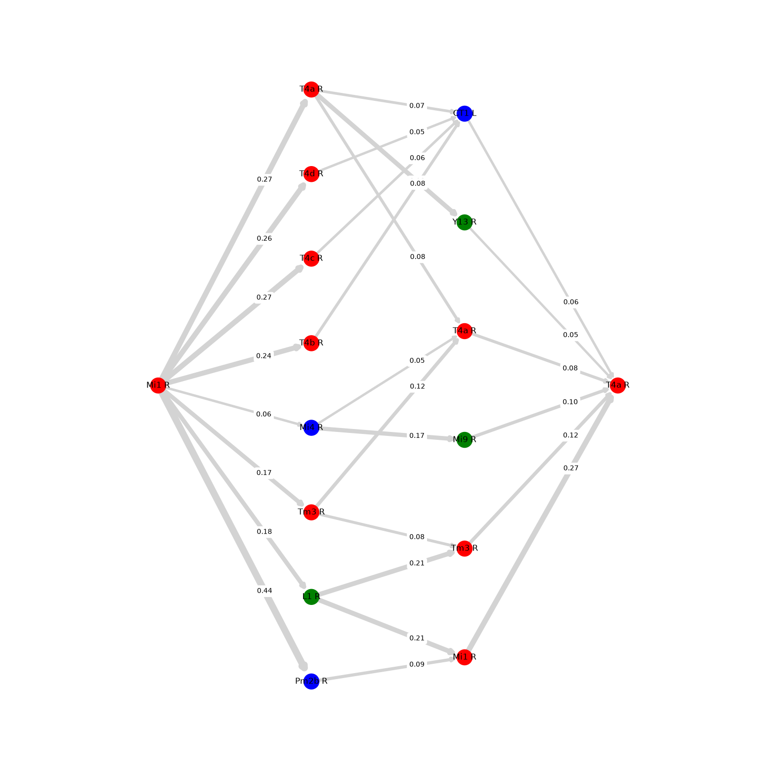
(None, None)To create an interactive visualisation, we can do the following:
# This creates an interactive plot using Pyvis.
# The interactive visualization is saved as paths.html in your current working directory (the folder where this notebook is running).
# Open paths.html in a web browser to explore the network!
plot_paths(paths_filt, edge_text=True, figsize=(20, 20), interactive=True)
paths.html
What does my data show me?
We can see that many of the intermediate neurons in these paths are cholinergic (red, acetylcholine), with some GABAergic (blue) and glutamatergic (green) cell-types also present.
Since Mi1 is cholinergic, we might expect its influence to be excitatory. However, it is important to remember that Mi1 and T4a are not directly synaptically connected in these 3-hop paths! If they were, we could interpret a direct Mi1 → T4a connection as excitatory based on Mi1’s neurotransmitter identity. Instead, the 3-hop paths contain multiple connections, and the neurotransmitter identity of each intermediate neuron provides information about the likely sign of the individual connections along the path. This allows us to consider how excitatory and inhibitory connections are combined across the pathway. Keep in mind that the input proportion on each edge and thickness of the edges describes the connection strength between that specific pair of neurons or cell types.
Looking at the input proportions, which connections appear to contribute the most input to T4a? Do these high input proportions correspond to high input proportions at the preceding step in the path? In other words, does a strong connection into T4a necessarily mean that the upstream neuron also receives a strong connection from its own upstream partner? How does this relate to your understanding of how we calculate effective connectivity?
What do you think is going on with Mi1 -> T4a, T4b, T4c, T4d -> CT1 -> T4a? Why would connections from Mi1 -> T4 subtypes be necessary? Why is T4a overrepresented in this plot? Is there anything else you notice that may have escaped my notice? These questions can serve as an anchor for your next analysis and help you explore the data further!
Also this would be a nice time to look at the functions of the cell types from the type_to_function dictionary. Are there some cell types functionally known / unknown in the pathway? Seeing this connectivity pathway what can you infer they are doing along with their NT identity?
Hexmaps
Let’s say now your curiosity leads you to ask: well, I now know how much influence a source cell type has on a target at different path lengths, and I know who the intermediate cell type players are. Now I want to know, spatially, is this influence the same across the visual field, or is it concentrated in particular spots?
In particular, this is a question we can explore using the fly visual system. The fly visual system contains approximately 800 ommatidia, which sample different locations in the animal’s visual field. You can think of each ommatidium as a small pixel in the fly’s view. Learn more about the optic lobes.
Visual neurons are perfect for this question because most cell types in the visual system sample the entire visual field, with approximately 800 neurons or more representing these different locations. This means we can ask:
Is effective connectivity concentrated in particular parts of the visual field? And if so, where in the visual field does the source most strongly influence the target?
A hexmap lets us look at this spatially. Here, we project the effective connectivity values associated with individual visual neurons onto the locations of the ommatidia that they represent. Each hexagon therefore corresponds to a small region of the fly’s visual field, allowing us to see whether the influence is spread across the visual field or concentrated in particular locations.
Keep in mind that these neuron locations or coordinates are not available for every neuron in the connectome. They come from the retinotopic (see here for what retinotopy is) coordinate systems developed for the fly visual system. For the female FAFB dataset, the coordinates were developed by Matsliah et al., 2024, while for the maleCNS visual system used here, the coordinates come from Nern et al., 2025.
For Nern et al., these coordinate systems are based on columnar visual neurons: repeating neuron types that occur across the visual field. The authors assigned coordinates to 15 such columnar cell types, including L1, L2, L3, L5, Mi1, Mi4, Mi9, C2, C3, Tm1, Tm2, Tm4, Tm9, Tm20 and T1. These neurons occur approximately once per retinotopic column, allowing their coordinates to correspond to locations on the fly’s compound eye. In simple terms, these cell types are repeated across almost the entire visual field, with around 800 copies of each cell type. Nern et al., assigned neurons to 892 hexagonal coordinates in the medulla (where columnar neurons tend to be).
Choosing the cell types to map
For this example, we will keep using the columnar Mi1 → T4a example we have been exploring to create these hex-maps. Let’s first filter for Mi1 cell types on the right side that have coordinates, and T4a cell types on the right side.
# Source: only neurons that have a column assignment
inidx = mcns_meta.idx[(mcns_meta.cell_type == 'Mi1') & (mcns_meta.somaSide == 'R') & (mcns_meta.coords.notna())]
outidx = mcns_meta.idx[(mcns_meta.cell_type == 'T4a') & (mcns_meta.somaSide == 'R')] # no na filtering here because only columnar neurons (such as Mi1) have coordinates.
Now, let’s make two dictionaries that connect each neuron’s index to its coordinates and body ID. The first dictionary lets us find where a neuron is located using its index. The second lets us find its body ID using the same index.
# make new dictionaries mapping index to coordinates in the visual system
mcns_idx_to_coords = dict(zip(mcns_meta.idx, mcns_meta.coords))
mcns_idx_to_bodyid = dict(zip(mcns_meta.idx, mcns_meta.bodyid))
Using find_paths_of_length, let’s query the 3-hop connectivity and input proportion strength between Mi1 and T4a.
hex_paths = find_paths_of_length(mcns_inprop, inidx, outidx, target_layer_number=3)
hex_pathsOur connections are currently organised by individual neurons. Let’s group these neurons by what we want to represent in our analysis.
For each path, group_paths lets us decide how to group our 3-hop connectivity dataframe from above.
pre_group→ how we group the source neuronsintermediate_group→ how we group the intermediate neuronspost_group→ how we group the target neurons
For our hexmap, we want to know where in the visual field the Mi1 → T4a influence is strongest. Therefore, we want to group our Mi1 source neurons by their visual-field coordinates:
For the intermediate and target neurons, we do not want to group them by visual-field location. Instead, we want to keep each individual neuron separate (as only columnar neurons have coordinates!). We can do this using their unique bodyid.
One important detail: if intermediate_group is not specified, it automatically uses pre_group. Since our pre_group is based on Mi1 coordinates, leaving it out would also group the intermediate neurons by coordinates. This is why we explicitly set intermediate_group=mcns_idx_to_bodyid here.
hex_paths_df = group_paths(hex_paths, pre_group=mcns_idx_to_coords, intermediate_group=mcns_idx_to_bodyid, post_group=mcns_idx_to_bodyid)
hex_paths_df# Using our 3-hop hex paths dataframe, lets calculate effective connectivity of Mi1 -> T4a.
# Pre is Mi1 in coordinates. Post is T4a bodyID labels from neuPrint (maleCNS)
ec_df = effective_conn_from_paths(hex_paths_df)
ec_dfGPU not available, using CPU instead.
fig = hex_heatmap(ec_df , dataset='mcns_right')
fig.show()# number of columns which are postID for T4a.
#These correspond to the number of neuron in a T4a cell type. Hence the slider is showing individual post T4a neurons.
len(ec_df.columns) 849Spatial organization of Mi1–T4a effective connectivity
Here, we visualize the effective connectivity from Mi1 neurons to individual T4a neurons across the visual field. Each hexagon represents a medulla column in the hexagonal coordinate system used to map the fly’s visual system. The position of each hexagon indicates where the Mi1 neuron is located in the visual-field map, while its colour represents the effective connectivity from that Mi1 to the selected T4a neuron.
The slider allows us to select different post-synaptic T4a neurons. As we change the selected T4a neuron, the spatial pattern of Mi1 effective connectivity shifts across the medulla map rather than just staying in one spot. Also notice that the connectivity is not concentrated in just one hexagon. Instead, it is strongest in a central hexagon and extends to several neighbouring hexagons, with weaker connectivity sometimes extending even further.
This raises an interesting question: if there are approximately as many T4 neurons (849 neurons) sas there are medulla columns, why couldn’t Nern et al. (2025) simply assign each T4a neuron to one medulla column? Look closely at the hexmap. If one medulla column corresponded to one T4a neuron, we might expect the input to each T4a neuron to be concentrated in a single hexagon. Instead, we see a cluster of several neighbouring hexagons. In this example, there is one strongly coloured central hexagon surrounded by approximately six neighbouring hexagons, with some weaker connectivity extending beyond them.
This is an important feature of T4 anatomy. Nern et al. (2025) used Mi1-T4 neurons to establish a coordinate system linking the medulla to the lobula plate. T4 neurons were particularly useful because they receive strong input from Mi1, their axons terminate in one of four lobula plate layers corresponding to the four cardinal motion directions, and there are approximately as many T4 neurons of each type as there are medulla columns.
However, T4 neurons cannot simply be assigned to a single medulla column. Their dendrites spread across several neighbouring columns, so each T4 neuron samples information from a local group of columns. Nern et al. used this anatomical information to determine the medulla coordinates associated with each T4 neuron. They could then apply those same coordinates to the T4 axons in the lobula plate, effectively using T4 neurons as a bridge between the two optic lobe regions. This allowed them to establish corresponding column coordinates between the medulla and lobula plate.
So, when you look at this hexmap, the multiple coloured hexagons, they reflect the underlying biology: a single T4a neuron integrates input from several neighbouring medulla columns. The hexmap therefore gives us an intuitive way to see the spatial extent of Mi1 input onto an individual T4a neuron. Look at edge-cases (at the edge of the eye), does anything change, why?