Tutorial 1 (Introductory): Visualizing Timeseries

Working with Timeseries Data¶

In this notebook, we will:

1. Load a CSV file from the ts/ folder inside our project directory

2. Inspect the data

3. Get the Schaefer atlas region names with nilearn

4. Subset one subject

5. Subset one brain region

6. Plot that region’s activity over time

Below, we’ll be importing some python packages that are required for this script. Common packages are

• numpy and pandas to deal with numbers and dataframes (i.e., tables)

• matplotlib for data visualization

• pathlib for managing your file paths/directories

• nilearn for anything to do with neuroimaging data

Feel free to run the code below to “import” these packages, which is a way to let the code knows that we’ll be using these specific packages.

1. Set Up the File Path¶

First, we will define the directory where this notebook is using the function or command “cwd” from the “Path” package that we have imported from above from pathlib import Path

cwd = current working directory

We’ll be calling this current working directory as your project directory.

Then, where your code is, create a folder called “ts”. Within this folder “ts”, we’ll store our timeseries file in Schaefer parcellation (schaefer100_timeseries_long.csv).

With this, try to understand what the code below is doing!

2. Load the CSV File¶

Next, we need to convert (or import) the csv file into a “dataframe” format.

A DataFrame is like a spreadsheet: rows and columns are organized in a table. Dataframes make it easy for us to manipulate large datasets with many rows and columns.

We use pandas.read_csv() to import the data into a DataFrame (i.e., read_csv function from the pandas package)

If you have imported the packages and indicated your file paths correctly, you should be able to run the code below.

3. Understand the Structure of the Dataframe¶

Now that we have imported the timeseries data from the csv into the dataframe format (stored in the timeseries_df variable), let’s try to make sense of our dataframe or the timeseries data!

Dimension¶

First, let’s check the shape or the dimension of the dataframe using .shape from pandas.

This returns: (143440, 101). Recall that a dataframe’s shape is reported as: (number_of_rows, number_of_columns). Therefore, our dataset contains 143,440 rows and 101 columns

The 101 columns consist of:

• 1 column containing the subject ID (subject)

• 100 columns containing brain activity values from the Schaefer100 atlas regions

The 143,440 rows contain data from all subjects combined.

Since this dataset contains 220 subjects, each with 652 fMRI time points, we have: 220 subjects × 652 time points = 143,440 rows

In other words, this CSV file stores the complete timeseries dataset for every participant in a single table.

Previewing Your Dataframe¶

Timeseries data from neuroimaging is often very large. However, we can use head from pandas to see the first few rows and some columns from our dataframe.

Using head(), we can see from the above that the first column contains the subject ID, while the remaining columns contain activity values from Schaefer100 brain regions (for example, 7Networks_LH_Vis_1, 7Networks_LH_Vis_2, and so on).

Each row represents a single fMRI time point from one subject:

• each row = one fMRI time point

• first column = subject identifier

• remaining columns = brain activity values for each Schaefer100 brain region

• consecutive rows for the same subject form that subject’s fMRI timeseries (we’ll be visualizing this timeseries later!)

Remember, all subjects are stored together in the same dataframe.

To gain some more intuition to this dataset, let’s do two things:

• get a list of column names and subject names

• extract the data just for a single subject and explore their timeseries before moving on to analyses involving the full dataset.

Each row represents a single fMRI time point from one subject:

• each row = one fMRI time point

• first column = subject identifier

• remaining columns = brain activity values for each Schaefer100 brain region

• consecutive rows for the same subject form that subject’s fMRI timeseries (we’ll be visualizing this timeseries later!)

Remember, all subjects are stored together in the same dataframe.

To gain some more intuition to this dataset, let’s do two things:

• get a list of column names and subject names

• extract the data just for a single subject and explore their timeseries before moving on to analyses involving the full dataset.

List of Brain Regions (Columns) and Subject Ids (Rows)¶

Columns (brain regions)

Recall that each column corresponds to either:

• the subject identifier (subject)

• a Schaefer100 brain region

The code below converts the dataframe’s column names into a Python list and prints them.

A list is one of Python’s basic data structures used to store multiple items in a specific order. You can think of a list like a numbered collection, where each item has a position and can be accessed individually.

For example, a list can store many brain region names, allowing us to access, inspect, or loop through them one at a time.

For the code below, all you need to know is that we are applying .tolist() to the dataframe to create a new list containing all their column names.

Obtaining list of unique subject IDs:

Let’s try to obtain a list of unique subject IDs.

The results from the print(column_names) show that the first column is the ‘subject’ column. (Remember, list stores values in a specific order).

The dataframe contains many rows for each subject because every subject has multiple fMRI time points.

For example, subject sub-010002 may appear 652 times because that participant has 652 time points.

If we simply print the subject column, we would see many repeated subject IDs. The output shown after printing the subject column shows that there are 143440 rows (Length: 143440).

So the next step is to find unique or distinct subject IDs that appear in subject_column.

In pandas, we can use .unique() to find distinct values in a single column, which is what we need to find distinct subject IDs that appear in subject_column.

4. Subset the Dataframe for One Subject¶

Right now, our dataframe contains the timeseries data for all 220 subjects. While this is ideal for large-scale analyses, it is often easier to understand the structure of the data by first examining a single participant.

Let’s extract all time points belonging to a single participant: sub-010003.

Because each row corresponds to one time point, the resulting dataframe will contain many rows (for example, ~652 rows) rather than a single row.

5. Extract a Single Brain Region Timeseries of a Subject¶

Now let’s focus on one brain region:

7Networks_LH_Vis_1

This region belongs to the left hemisphere visual network.

By selecting this column from our subject dataframe, we obtain a single timeseries showing how activity in this region changes over time.

6. Visualize the Timeseries¶

We can now visualize how activity changes over time in this brain region.

The x-axis represents fMRI time points.

The y-axis represents the activity value recorded for this brain region at each time point.

We’ll be using matplotlib to plot our data.

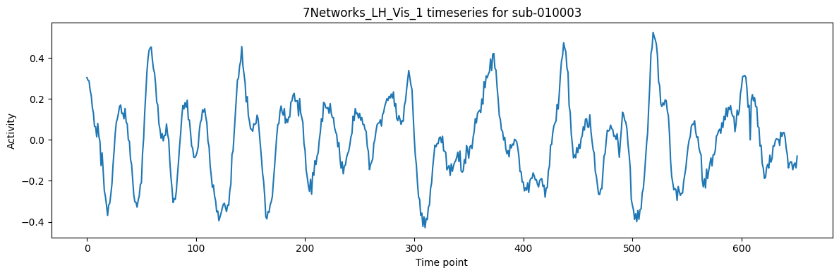
Understanding the plot¶

The plot() function draws a line connecting the activity values recorded at each time point.

In this figure:

• the x-axis represents time points in the fMRI scan

• the y-axis represents activity in the selected brain region

• each point on the line corresponds to one row in the subject’s timeseries dataframe

Notice how the signal rises and falls over time. These fluctuations are the fMRI signal measured from this brain region. Later, we will compare these fluctuations across different brain regions to estimate functional connectivity.