Tutorial 2 (Introductory): Functional Connectivity - 2026–2027 Connectomics Research Competition

In the previous “Tutorial 1: Visualizing Timeseries”, you’ve learned how to load, inspect, subset, and visualize timeseries data.

Now, we can take the next step and calculate functional connectivity (FC). In this notebook, we will use the same Schaefer100 timeseries CSV file and learn how to compute FC for one subject, summarize FC across all subjects, save the results, and load them back later.

Calculating Functional Connectivity¶

In this notebook, we will:

Load the Schaefer100 timeseries CSV file from the ts/ folder inside our project directory
Calculate functional connectivity for one subject
Visualize that subject’s FC matrix in a static way with Matplotlib and in an interactive way with Plotly
Calculate the mean FC across all subjects
Save the full 3D stack of subject-level FC matrices in the results/ folder
Load the saved array again and extract the FC matrix for a single subject

Below, we’ll import the Python packages that we need for this notebook.

Pathlib helps us work with file paths and folders
NumPy helps us work with arrays and numerical calculations
Pandas helps us work with tabular data
Matplotlib helps us create static plots
Plotly helps us create interactive plots
Nilearn helps us access neuroimaging resources such as the Schaefer atlas labels

Feel free to run the code below to import these packages before moving on.

from pathlib import Path

import numpy as np
import pandas as pd
import matplotlib.pyplot as plt

import plotly.graph_objects as go
import plotly.io as pio
pio.renderers.default = "browser"


from nilearn.datasets import fetch_atlas_schaefer_2018

1. Set up the file paths¶

We will use the same folder style as Tutorial 1.

The main project directory is stored in PROJECT_DIR. Inside that directory, we will look for the ts/ folder that contains the timeseries CSV file. Later, we will also create a results/ folder where we will save the FC matrices that we compute in this notebook.

If this notebook lives inside your project directory, Path.cwd() is usually the easiest option because it automatically points to the current working directory.

# Option 1: use the current working directory if the notebook lives inside the project folder
# PROJECT_DIR = Path.cwd()

# Option 2: manually specify your project directory if needed
PROJECT_DIR = Path("/Users/shemrock/Library/CloudStorage/OneDrive-Nexus365/Clematis/guide/Conn_comp/competition2026/lemon2026") # assign the main directory containing your data to the PROJECT_DIR variable

TS_DIR = PROJECT_DIR / "ts" # ts stands for timeseries
RESULTS_DIR = PROJECT_DIR / "results"
CSV_FILE = TS_DIR / "schaefer100_timeseries_long.csv"

# Make sure the results folder exists so we can save outputs there later
RESULTS_DIR.mkdir(parents=True, exist_ok=True)

print("Project directory:", PROJECT_DIR)
print("Timeseries file:", CSV_FILE)
print("Results directory:", RESULTS_DIR)

Project directory: /Users/shemrock/Library/CloudStorage/OneDrive-Nexus365/Clematis/guide/Conn_comp/competition2026/lemon2026
Timeseries file: /Users/shemrock/Library/CloudStorage/OneDrive-Nexus365/Clematis/guide/Conn_comp/competition2026/lemon2026/ts/schaefer100_timeseries_long.csv
Results directory: /Users/shemrock/Library/CloudStorage/OneDrive-Nexus365/Clematis/guide/Conn_comp/competition2026/lemon2026/results

2. Load the CSV file¶

Next, we import the CSV file into a pandas DataFrame.

A DataFrame is like a spreadsheet: it stores data in rows and columns, and it is one of the most useful data structures for data science and neuroimaging work in Python.

Here, each row is one fMRI time point for one subject, and each column is either the subject ID or a brain region from the Schaefer100 atlas.

timeseries_df = pd.read_csv(CSV_FILE)

print("Shape of dataframe:", timeseries_df.shape)
timeseries_df.head()

Shape of dataframe: (143440, 101)

3. Understand the structure of the dataframe¶

Let’s revise how our dataframe looks like! First, let’s look at the shape of the dataframe:

print(timeseries_df.shape)

This returns the number of rows and the number of columns.

In this dataset, the shape tells us that we have:

143,440 rows
101 columns

The 101 columns consist of:

1 column containing the subject ID (subject)
100 columns containing brain activity values from the Schaefer100 atlas regions

The 143,440 rows contain data from all subjects combined.

Since this dataset contains 220 subjects, each with 652 fMRI time points, we have:

220 subjects × 652 time points = 143,440 rows

In other words, this CSV file stores the complete timeseries dataset for every participant in a single table.

Because all subjects are stored together, a common first step is to identify the columns that contain the brain region timeseries and the subject IDs that appear in the dataset.

# Get a Python list of all column names in the dataframe
column_names = timeseries_df.columns.tolist()

# Show the column names
print(column_names)

# Get a Python list of all unique subject IDs
subject_ids = timeseries_df["subject"].unique().tolist()

# Show how many subjects are in the dataset
print("Number of unique subjects:", len(subject_ids))
print("First five subject IDs:", subject_ids[:5])

# Get the brain region columns only (everything except the subject column)
region_cols = [col for col in column_names if col != "subject"]

print("Number of region columns:", len(region_cols))
print("First five region names:", region_cols[:5])

['subject', '7Networks_LH_Vis_1', '7Networks_LH_Vis_2', '7Networks_LH_Vis_3', '7Networks_LH_Vis_4', '7Networks_LH_Vis_5', '7Networks_LH_Vis_6', '7Networks_LH_Vis_7', '7Networks_LH_Vis_8', '7Networks_LH_Vis_9', '7Networks_LH_SomMot_1', '7Networks_LH_SomMot_2', '7Networks_LH_SomMot_3', '7Networks_LH_SomMot_4', '7Networks_LH_SomMot_5', '7Networks_LH_SomMot_6', '7Networks_LH_DorsAttn_Post_1', '7Networks_LH_DorsAttn_Post_2', '7Networks_LH_DorsAttn_Post_3', '7Networks_LH_DorsAttn_Post_4', '7Networks_LH_DorsAttn_Post_5', '7Networks_LH_DorsAttn_Post_6', '7Networks_LH_DorsAttn_PrCv_1', '7Networks_LH_DorsAttn_FEF_1', '7Networks_LH_SalVentAttn_ParOper_1', '7Networks_LH_SalVentAttn_FrOperIns_1', '7Networks_LH_SalVentAttn_FrOperIns_2', '7Networks_LH_SalVentAttn_PFCl_1', '7Networks_LH_SalVentAttn_Med_1', '7Networks_LH_SalVentAttn_Med_2', '7Networks_LH_SalVentAttn_Med_3', '7Networks_LH_Limbic_OFC_1', '7Networks_LH_Limbic_TempPole_1', '7Networks_LH_Limbic_TempPole_2', '7Networks_LH_Cont_Par_1', '7Networks_LH_Cont_PFCl_1', '7Networks_LH_Cont_pCun_1', '7Networks_LH_Cont_Cing_1', '7Networks_LH_Default_Temp_1', '7Networks_LH_Default_Temp_2', '7Networks_LH_Default_Par_1', '7Networks_LH_Default_Par_2', '7Networks_LH_Default_PFC_1', '7Networks_LH_Default_PFC_2', '7Networks_LH_Default_PFC_3', '7Networks_LH_Default_PFC_4', '7Networks_LH_Default_PFC_5', '7Networks_LH_Default_PFC_6', '7Networks_LH_Default_PFC_7', '7Networks_LH_Default_pCunPCC_1', '7Networks_LH_Default_pCunPCC_2', '7Networks_RH_Vis_1', '7Networks_RH_Vis_2', '7Networks_RH_Vis_3', '7Networks_RH_Vis_4', '7Networks_RH_Vis_5', '7Networks_RH_Vis_6', '7Networks_RH_Vis_7', '7Networks_RH_Vis_8', '7Networks_RH_SomMot_1', '7Networks_RH_SomMot_2', '7Networks_RH_SomMot_3', '7Networks_RH_SomMot_4', '7Networks_RH_SomMot_5', '7Networks_RH_SomMot_6', '7Networks_RH_SomMot_7', '7Networks_RH_SomMot_8', '7Networks_RH_DorsAttn_Post_1', '7Networks_RH_DorsAttn_Post_2', '7Networks_RH_DorsAttn_Post_3', '7Networks_RH_DorsAttn_Post_4', '7Networks_RH_DorsAttn_Post_5', '7Networks_RH_DorsAttn_PrCv_1', '7Networks_RH_DorsAttn_FEF_1', '7Networks_RH_SalVentAttn_TempOccPar_1', '7Networks_RH_SalVentAttn_TempOccPar_2', '7Networks_RH_SalVentAttn_FrOperIns_1', '7Networks_RH_SalVentAttn_Med_1', '7Networks_RH_SalVentAttn_Med_2', '7Networks_RH_Limbic_OFC_1', '7Networks_RH_Limbic_TempPole_1', '7Networks_RH_Cont_Par_1', '7Networks_RH_Cont_Par_2', '7Networks_RH_Cont_PFCl_1', '7Networks_RH_Cont_PFCl_2', '7Networks_RH_Cont_PFCl_3', '7Networks_RH_Cont_PFCl_4', '7Networks_RH_Cont_Cing_1', '7Networks_RH_Cont_PFCmp_1', '7Networks_RH_Cont_pCun_1', '7Networks_RH_Default_Par_1', '7Networks_RH_Default_Temp_1', '7Networks_RH_Default_Temp_2', '7Networks_RH_Default_Temp_3', '7Networks_RH_Default_PFCv_1', '7Networks_RH_Default_PFCv_2', '7Networks_RH_Default_PFCdPFCm_1', '7Networks_RH_Default_PFCdPFCm_2', '7Networks_RH_Default_PFCdPFCm_3', '7Networks_RH_Default_pCunPCC_1', '7Networks_RH_Default_pCunPCC_2']
Number of unique subjects: 220
First five subject IDs: ['sub-010002', 'sub-010003', 'sub-010004', 'sub-010005', 'sub-010006']
Number of region columns: 100
First five region names: ['7Networks_LH_Vis_1', '7Networks_LH_Vis_2', '7Networks_LH_Vis_3', '7Networks_LH_Vis_4', '7Networks_LH_Vis_5']

4. Brief introduction to Nilearn and extracting Schaefer100 brain regions¶

Fetching Schaefer Atlas¶

In the previous tutorial, the names of the Schaefer100 brain regions were labeled in our timeseries dataframe. However, we can also ask Nilearn to download information about the Schaefer atlas for us.

To do this, we use the function fetch_atlas_schaefer_2018() from the nilearn package.

A function is a reusable piece of code that performs a specific task. In this case, the function downloads (or loads, if it has already been downloaded) the Schaefer atlas and returns information about it.

Notice below that we provide three arguments inside the parentheses:

n_rois=100 requests the 100-region version of the atlas.
yeo_networks=7 requests the 7-network organization of those regions.
resolution_mm=2 requests the atlas at 2 mm resolution

# Fetch the Schaefer atlas labels for reference
schaefer = fetch_atlas_schaefer_2018(n_rois=100, yeo_networks=7, resolution_mm=2)

[fetch_atlas_schaefer_2018] Dataset found in /Users/shemrock/nilearn_data/schaefer_2018

The function returns an object containing several pieces of information about the atlas, including the atlas image, file locations, and the names of every brain region.

When you work with Python packages like Nilearn, NumPy, Pandas, or Matplotlib, it is always a good idea to check the official documentation for each function. The documentation usually explains what the function does, what arguments it accepts, and what it returns. For this example, you can look up fetch_atlas_schaefer_2018() in the Nilearn documentation.

For example, the Nilearn documentation for this function is here:

fetch_atlas_schaefer_2018() in the Nilearn docs.

Documentations¶

If we look at the documentation for fetch_atlas_schaefer_2018(), there are two sections that are especially useful:

PARAMETERS

The Parameters section describes the arguments that we can pass into the function. These allow us to customize how the function behaves.

For example, we specify:

n_rois=100 to request the Schaefer atlas with 100 brain regions.
yeo_networks=7 to use the 7-network organization.
resolution_mm=2 to use the atlas at 2 mm resolution.

Whenever you use a new Python function, the Parameters section is the first place to look if you want to understand what inputs the function accepts.

RETURNS

The Returns section tells us what the function gives back after it finishes running.

For fetch_atlas_schaefer_2018(), the function returns an object containing several pieces of information about the Schaefer atlas. One of these is labels, which is a list of strings containing the names of all 100 brain regions.

We can access these labels using dot notation:

atlas_labels = schaefer.labels

atlas_labels = schaefer.labels

print("Number of atlas labels returned by nilearn:", len(atlas_labels))
print("First ten atlas labels:", atlas_labels[:10])

Number of atlas labels returned by nilearn: 101
First ten atlas labels: ['Background', '7Networks_LH_Vis_1', '7Networks_LH_Vis_2', '7Networks_LH_Vis_3', '7Networks_LH_Vis_4', '7Networks_LH_Vis_5', '7Networks_LH_Vis_6', '7Networks_LH_Vis_7', '7Networks_LH_Vis_8', '7Networks_LH_Vis_9']

Notice that there are 101 labels rather than 100. This is because the first label corresponds to the background (index 0), which does not represent a brain region. It is simply a placeholder for locations that are not assigned to any Schaefer brain region such as empty space surrounding the brain in the image. The remaining 100 labels correspond to the 100 Schaefer brain regions used in our analyses.

5. Calculate functional connectivity for one subject¶

Functional connectivity, or FC, describes how strongly the activity patterns of two brain regions are related over time.

In this notebook, we will use the most common measure of FC: the Pearson correlation between the timeseries of every pair of brain regions.

Recall that our subject’s timeseries dataframe contains:

one row for each fMRI time point
one column for each brain region

To calculate FC, we compare the timeseries of every brain region with every other brain region by computing their Pearson correlation.

The result is an FC matrix:

the rows and columns both represent the brain regions
each cell contains the correlation between two brain regions
the diagonal is 1, because every region is perfectly correlated with itself
the matrix is symmetric, because the correlation between region A and region B is the same as between region B and region A

We will start by calculating the FC matrix for a single subject so that the process is easy to understand before extending it to the entire dataset.

Subsetting a dataframe for a single subject¶

## Subsetting a dataframe for a single subject (similar to tutorial1)

# Choose a sample subject
subject_id = "sub-010003"

# Keep only the rows that belong to the selected subject
sub_df = timeseries_df[timeseries_df["subject"] == subject_id].copy()

# Reset the row index so the subject's time points start at 0
sub_df = sub_df.reset_index(drop=True)

print("Shape of subject dataframe:", sub_df.shape)
sub_df.head()

Shape of subject dataframe: (652, 101)

# Keep only the brain-region columns for this subject
subject_timeseries = sub_df[region_cols]

# Create a new dataframe containing only the brain-region columns 
subject_timeseries = sub_df.drop(columns="subject") # dropping specific columns using .drop in pandas

# Previewing subject_timeseries
subject_timeseries

Using .corr() to compute FC (pairwise correlation)¶

# Calculate the FC matrix by correlating every region with every other region
subject_fc = subject_timeseries.corr()

print("Shape of subject FC matrix:", subject_fc.shape)
subject_fc.iloc[:5, :5]

Shape of subject FC matrix: (100, 100)

Using Nilearn to calculate FC¶

Instead of computing correlations manually, we can use Nilearn’s built-in ConnectivityMeasure class.

A class is like a blueprint for creating an object that can perform a task. Here, ConnectivityMeasure is designed specifically for connectome calculations, such as correlation-based functional connectivity.

We tell it that we want correlation-based FC by setting:

kind="correlation"

Then we give it the subject’s timeseries data.

Important: ConnectivityMeasure.fit_transform() expects a list of arrays, where each array is one subject’s timeseries matrix.

For one subject, the input should look like this:

rows = time points
columns = brain regions

The output is a 3D array with shape:

(n_subjects, n_regions, n_regions)

So if we give it one subject, the result will have shape (1, 100, 100).

from nilearn.connectome import ConnectivityMeasure

# Create a correlation-based connectivity estimator
correlation_measure = ConnectivityMeasure(kind="correlation", verbose=1)

The fit_transform() function is designed to calculate functional connectivity for one or more subjects.

It expects a list, where each element is a 2D array containing one subject’s timeseries data.

Since we currently have only one subject, we simply place that subject’s timeseries inside a list:

[subject_timeseries.to_numpy()]

# subject_timeseries should contain only the brain-region columns
correlation_matrix = correlation_measure.fit_transform([subject_timeseries.to_numpy()])

print(correlation_matrix.shape)

[ConnectivityMeasure.wrapped] Finished fit
(1, 100, 100)

/var/folders/ct/7zc2pz097mq7rktbqqr2_29m0000gn/T/ipykernel_37899/4055317337.py:2: FutureWarning: The default strategy for standardize is currently 'zscore' which incorrectly uses population std to calculate sample zscores. The new strategy 'zscore_sample' corrects this behavior by using the sample std. In release 0.14.0, the default strategy will be replaced by the new strategy, the 'zscore' option will be removed. and using standardize=True will fall back to 'zscore_sample'.To avoid this warning, please use 'zscore_sample' instead.
  correlation_matrix = correlation_measure.fit_transform([subject_timeseries.to_numpy()])

6. Visualize FC for one subject with Matplotlib¶

Although the FC matrix is simply a table of correlation values, it is much easier to interpret when displayed as a heatmap.

A heatmap uses colors to represent numerical values. In our FC matrix:

each row and column corresponds to a brain region
each square represents the correlation between a pair of brain regions
warmer colors (red) indicate stronger positive correlations
cooler colors (blue) indicate negative correlations
white or light colors indicate correlations close to zero

We will first create a static heatmap using Matplotlib, one of the most widely used plotting libraries in Python.

But before that, let’s make sure we prep our correlation_matrix, which contains a 100 x 100 FC of a single subject. Also remember, it has a shape of (1, 100, 100).

Since it contains one FC matrix, we simply need to extract the first (and only) matrix:

subject_fc = correlation_matrix[0]

subject_fc = correlation_matrix[0]

Now let’s plot the figure! Read the comments below.

# Create a new figure (plotting canvas)
# figsize=(9, 8) makes the figure 9 inches wide and 8 inches tall
plt.figure(figsize=(9, 8))

# Display the functional connectivity (FC) matrix as a heatmap
# - subject_fc is the 100 × 100 matrix of correlation values
# - vmin and vmax fix the color scale between -1 and 1 since those are the min and max correlation values possible
# - cmap="coolwarm" maps negative correlations to blue and positive correlations to red
# - origin="lower" places the first brain region in the bottom-left corner
plt.imshow(subject_fc, vmin=-1, vmax=1, cmap="coolwarm", origin="lower")

# Add a color bar to show how colors correspond to correlation values
plt.colorbar(label="Correlation")

# Add a title describing what is being displayed
# The f-string automatically inserts the subject ID into the title
plt.title(f"Functional connectivity for {subject_id}")

# Label the x-axis and y-axis
# Both axes represent the same set of brain regions
plt.xlabel("Brain region")
plt.ylabel("Brain region")

# Adjust the layout so labels and the color bar fit neatly within the figure
plt.tight_layout()

# Display the completed figure
plt.show()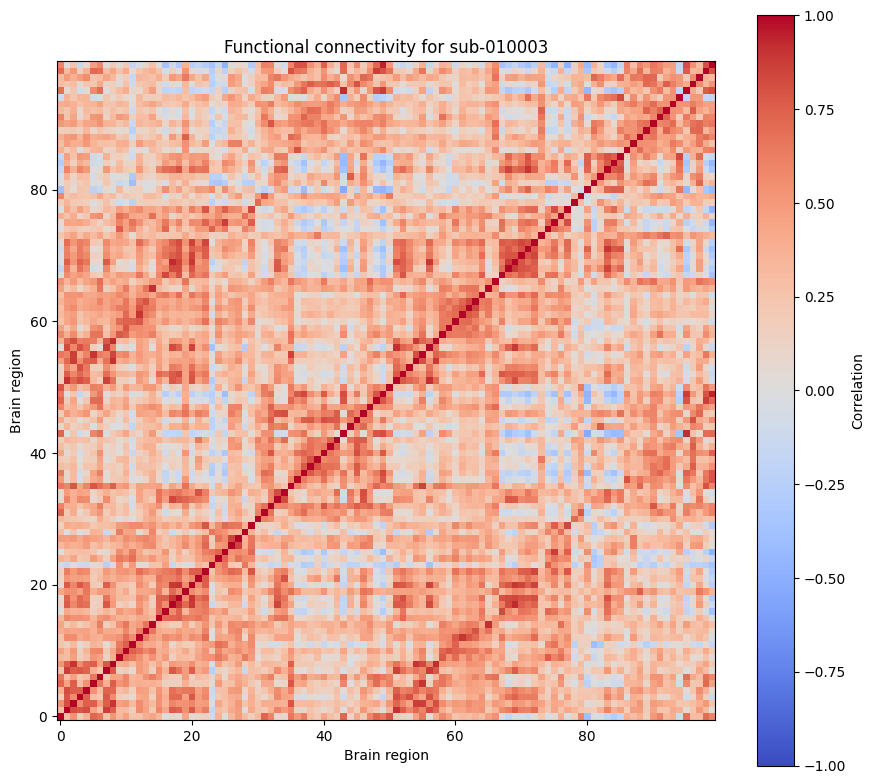

7. Visualize FC for one subject with Plotly¶

Plotly gives us an interactive version of the same FC matrix.

With the interactive heatmap, students can hover over cells, zoom in, and inspect values more closely.

First, let’s get the region labels from our atlas_labels. However, since our atlas_labels (obtained from the Nilearn’s Schaefer100 atlas) has the background, let’s remove the background label.

# Remove the background label
region_labels = atlas_labels[1:]

Now let’s use plotly!

We have already imported the plotly.io module and set the default renderer as the browser.

import plotly.io as pio
pio.renderers.default = "browser"

Here, plotly.io contains functions for displaying and saving Plotly figures. By setting the default renderer to "browser", every time we call fig.show(), Plotly will open the figure in your default web browser instead of displaying it inside the notebook.

Viewing the figure in a browser provides a larger workspace, making it much easier to explore the functional connectivity matrix interactively.

# Create a new Plotly figure containing a heatmap
fig = go.Figure(

    # The Heatmap object specifies what to draw
    data=go.Heatmap(

        # z contains the values to display (the FC matrix)
        z=subject_fc,

        # x and y provide the brain region names
        # These names will appear when hovering over the heatmap
        x=region_labels,
        y=region_labels,

        # Use a red-white-blue color scale
        # Blue = negative correlation, Red = positive correlation
        colorscale="RdBu_r",

        # Fix the color scale between -1 and 1
        # so different subjects can be compared fairly
        zmin=-1,
        zmax=1,

        # Label the color bar
        colorbar=dict(title="Correlation (r)"),
    )
)

# Update the appearance of the figure
fig.update_layout(

    # Add a title
    title=f"Functional connectivity for {subject_id}",

    # Axis titles
    xaxis_title="Brain region",
    yaxis_title="Brain region",

    # Set figure size (pixels)
    width=800,
    height=800,
)

# Hide the tick labels because there are too many brain regions
# The region names are still available when hovering over the heatmap
fig.update_xaxes(showticklabels=False)
fig.update_yaxes(showticklabels=False)

# Display the interactive figure
# fig.show() 
fig.show(renderer="notebook")

8. Calculate the mean FC across all subjects¶

Preparing the data for Nilearn¶

Earlier, we calculated the functional connectivity (FC) matrix for a single subject by giving Nilearn that subject’s timeseries.

Now we want to calculate FC for all 220 subjects.

To do this, we first need to prepare the data in a format that Nilearn expects. Specifically, ConnectivityMeasure.fit_transform() expects a list, where each element is the timeseries matrix for one subject.

Our goal is therefore to:

Loop through every subject in the dataset.
Extract that subject’s timeseries data.
Remove the subject column, keeping only the brain-region activity values.
Store each subject’s timeseries matrix in a list.

After the loop finishes, the list will contain 220 timeseries matrices—one for each subject—which we can then pass to Nilearn to calculate FC for the entire dataset in a single step.

# Create a Nilearn connectivity object that calculates correlation-based FC
correlation_measure = ConnectivityMeasure(kind="correlation", verbose=0)

# Get the list of all subject IDs
subject_ids = timeseries_df["subject"].unique().tolist()

# Keep only the brain-region column names
region_cols = timeseries_df.columns.drop("subject")

# Create an empty list that will store one timeseries matrix for each subject
subject_timeseries_list = []

# Loop through every subject ID in the dataset
for subj in subject_ids:

    # Select only the rows belonging to the current subject
    subj_df = timeseries_df[timeseries_df["subject"] == subj].copy()

    # Remove the "subject" column so only brain-region timeseries remain
    subj_timeseries = subj_df.drop(columns="subject").to_numpy()

    # Add this subject's timeseries matrix to our list
    subject_timeseries_list.append(subj_timeseries)

Now, the data structure of our subject_timeseries_list is as follows:

subject_timeseries_list │ ├── Subject 1 → (652 × 100) ├── Subject 2 → (652 × 100) ├── Subject 3 → (652 × 100) │ ⋮ │ └── Subject 220 → (652 × 100)

# Check how many items/matrices are in subject_timeseries_list
print(f"Number of subjects: {len(subject_timeseries_list)}") # 220

# For each matrix/subject, what's the shape?
print(f"Shape of first subject: {subject_timeseries_list[0].shape}") # 652 timepoints x 100 regions

Number of subjects: 220
Shape of first subject: (652, 100)

Calculate functional connectivity for every subject¶

Now that our data are stored in the format expected by Nilearn, we can calculate the FC matrices.

The fit_transform() function processes every subject in subject_timeseries_list and computes one FC matrix for each subject.

The result is a 3D NumPy array, where:

the first dimension indexes the subject
the second dimension indexes the first brain region
the third dimension indexes the second brain region

In our case, we will get a 220 subjects x 100 regions x 100 regions. In other words, the resulting array contains 220 subjects’ 100 x 100 FC matrix.

# Calculate one FC matrix per subject for all subjects
fc_stack = correlation_measure.fit_transform(subject_timeseries_list)

# Display the shape of the resulting 3D array
print("Shape of 3D FC stack:", fc_stack.shape)

Shape of 3D FC stack: (220, 100, 100)

The output should be:

(220, 100, 100)

This tells us that:

there are 220 subjects
each subject has a 100 × 100 functional connectivity matrix

We can think of this as a stack of FC matrices—one matrix for each participant in the study.

Calculate the mean functional connectivity matrix¶

Once fit_transform() has finished, Nilearn also computes the mean functional connectivity matrix across all subjects.

This matrix represents the average functional connectivity between every pair of brain regions in the dataset.

# Retrieve the mean FC matrix computed by Nilearn
mean_fc = correlation_measure.mean_

print(f"Mean correlation matrix has shape {mean_fc.shape}.")

Mean correlation has shape (100, 100).

The mean FC matrix is stored as a NumPy array.

To make it easier to inspect, we can convert it into a Pandas DataFrame and assign the Schaefer brain region names as the row and column labels.

# Turn the mean FC into a dataframe so it keeps region labels
mean_fc_df = pd.DataFrame(mean_fc, index=region_cols, columns=region_cols)

print("Shape of mean FC matrix:", mean_fc_df.shape)
mean_fc_df.iloc[:5, :5]

Shape of mean FC matrix: (100, 100)

9. Visualize the mean FC matrix¶

The mean FC matrix is a group-level summary of the dataset.

This helps us see which connections are consistently strong or weak across participants.

Let’s try plotting this using matplotlib like before!

plt.figure(figsize=(9, 8))

plt.imshow(mean_fc_df.values, vmin=-1, vmax=1, cmap="coolwarm", origin="lower")
plt.colorbar(label="Correlation")
plt.title("Mean functional connectivity across all subjects")
plt.xlabel("Brain region")
plt.ylabel("Brain region")
plt.tight_layout()
plt.show()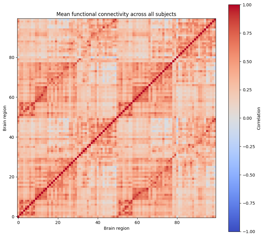

We can also use plotly!

fig = go.Figure(
    data=go.Heatmap(
        z=mean_fc_df.values,
        x=mean_fc_df.columns,
        y=mean_fc_df.index,
        colorscale="RdBu_r",
        zmin=-1,
        zmax=1,
        colorbar=dict(title="r"),
    )
)

fig.update_layout(
    title="Mean functional connectivity across all subjects",
    xaxis_title="Brain region",
    yaxis_title="Brain region",
    width=800,
    height=800,
)

# Hide the tick labels because there are too many brain regions
# The region names are still available when hovering over the heatmap
fig.update_xaxes(showticklabels=False)
fig.update_yaxes(showticklabels=False)
# fig.show

fig.show(renderer="notebook")

10. Save the FC results to computer¶

Once we have computed the FC matrices, we may want to save them so that we do not have to recompute them every time.

We will save:

the full 3D FC stack
the list of subject IDs
the list of region names
the mean FC matrix

Saving the subject IDs and region names is important because a raw NumPy array does not store the labels by itself.

# Define file names in the results folder
fc_stack_path = RESULTS_DIR / "subject_fc_stack.npy"
subject_ids_path = RESULTS_DIR / "subject_ids.npy"
region_names_path = RESULTS_DIR / "region_names.npy"
mean_fc_path = RESULTS_DIR / "mean_fc.npy"

# Save the arrays
np.save(fc_stack_path, fc_stack)
np.save(subject_ids_path, np.array(subject_ids))
np.save(region_names_path, np.array(region_cols))
np.save(mean_fc_path, mean_fc)

print("Saved:", fc_stack_path)
print("Saved:", subject_ids_path)
print("Saved:", region_names_path)
print("Saved:", mean_fc_path)

Saved: /Users/shemrock/Library/CloudStorage/OneDrive-Nexus365/Clematis/guide/Conn_comp/competition2026/lemon2026/results/subject_fc_stack.npy
Saved: /Users/shemrock/Library/CloudStorage/OneDrive-Nexus365/Clematis/guide/Conn_comp/competition2026/lemon2026/results/subject_ids.npy
Saved: /Users/shemrock/Library/CloudStorage/OneDrive-Nexus365/Clematis/guide/Conn_comp/competition2026/lemon2026/results/region_names.npy
Saved: /Users/shemrock/Library/CloudStorage/OneDrive-Nexus365/Clematis/guide/Conn_comp/competition2026/lemon2026/results/mean_fc.npy

11. Load the saved FC array again¶

A major advantage of saving the results is that we can load them again later without recalculating everything.

This is especially useful when the dataset is large or when the FC calculation takes a long time.

# Load the saved arrays from disk
loaded_fc_stack = np.load(fc_stack_path, allow_pickle=True)
loaded_subject_ids = np.load(subject_ids_path, allow_pickle=True)
loaded_region_names = np.load(region_names_path, allow_pickle=True)

print("Loaded FC stack shape:", loaded_fc_stack.shape)
print("Loaded subject IDs shape:", loaded_subject_ids.shape)
print("Loaded region names shape:", loaded_region_names.shape)

Loaded FC stack shape: (220, 100, 100)
Loaded subject IDs shape: (220,)
Loaded region names shape: (100,)

12. Extract the FC matrix for one subject from the saved array¶

Because the 3D array stores the subjects in a specific order, we first need to find the position of the subject we want.

Then we can use that index to pull out the correct 100 by 100 FC matrix.

# Convert the loaded subject IDs to a Python list so we can use .index()
loaded_subject_ids_list = loaded_subject_ids.tolist()

# Find the position of our sample subject 'sub-010003' that we have used previously to calculate an FC
subject_index = loaded_subject_ids_list.index('sub-010003')
print("Index of subject in saved array:", subject_index)

# Extract that subject's FC matrix from the 3D stack
subject_fc_loaded = loaded_fc_stack[subject_index]
print("Shape of loaded subject FC matrix:", subject_fc_loaded.shape)

Index of subject in saved array: 1
Shape of loaded subject FC matrix: (100, 100)

# Put the loaded matrix back into a dataframe with labels
subject_fc_loaded_df = pd.DataFrame(
    subject_fc_loaded,
    index=loaded_region_names,
    columns=loaded_region_names,
)

subject_fc_loaded_df.iloc[:5, :5]

13. Visualize the loaded subject FC matrix¶

This final step shows that the saved array can be used just like the original FC matrix.

That means we can load the data back from disk and continue analyzing it whenever we need to.

plt.figure(figsize=(9, 8))

plt.imshow(subject_fc_loaded_df.values, vmin=-1, vmax=1, cmap="coolwarm", origin="lower")
plt.colorbar(label="Correlation")
plt.title(f"Loaded functional connectivity for {subject_id}")
plt.xlabel("Brain region")
plt.ylabel("Brain region")
plt.tight_layout()
plt.show()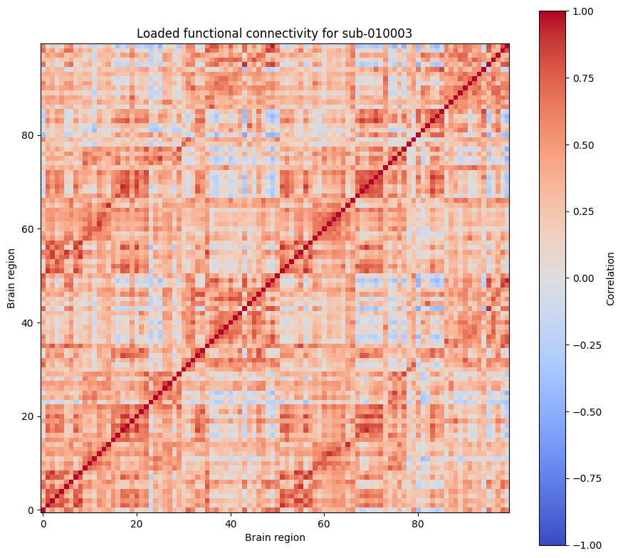

Summary¶

In this notebook, we learned how to:

compute FC for one subject
display FC as a static heatmap and an interactive Plotly figure
calculate the mean FC across all subjects
save the full subject-level FC stack as a 3D NumPy array
load the saved array back from disk
recover the FC matrix for a chosen subject

This gives us a complete FC workflow that starts from the Schaefer100 timeseries CSV file and ends with saved group-level and subject-level connectivity matrices.